Abstract

If there were no variations in distribution load, system voltage regulation would be a simple task.  But Ohm’s law dictates that a change in load produces a change in delivered voltage, and individual loads are constantly switching or varying.  While each specific load is difficult to predict, in aggregate the combined circuit load usually follows a repeatable daily trend.  In many areas, adjusting load tap changers or voltage regulators based on known load patterns is required for good regulation.  The Daily Profile graph, available in ProVision, is designed to make identifying these daily patterns as easy as possible.  This graph and some voltage regulation examples are described here.

Daily Profile Operation

A PMI Daily Profile is a graph with a 24 hour time span.  The recorder keeps 96 “bins”, one for each 15 minute period of a 24 hour day.  Throughout the recording session, the average value of each quantity (e.g. RMS voltage) is added to the applicable 15 minute bin.  As the recorder continues to accumulate data over days, the 24 hour composite graph becomes more representative of the average daily trend.  A large number of days in the average helps smooth out individual variations from day to day, and remove isolated events.

There is one Daily Profile graph for RMS voltage, current, real, reactive and apparent power, and THD.  Each graph contains the profile for all measured channels.  All Daily Profiles are recorded even if the corresponding stripchart measurement is disabled.  For example, Voltage and Current THD Profiles are available even without THD or harmonics enabled (provided that the recorder is capable of computing harmonics).

Voltage Regulation

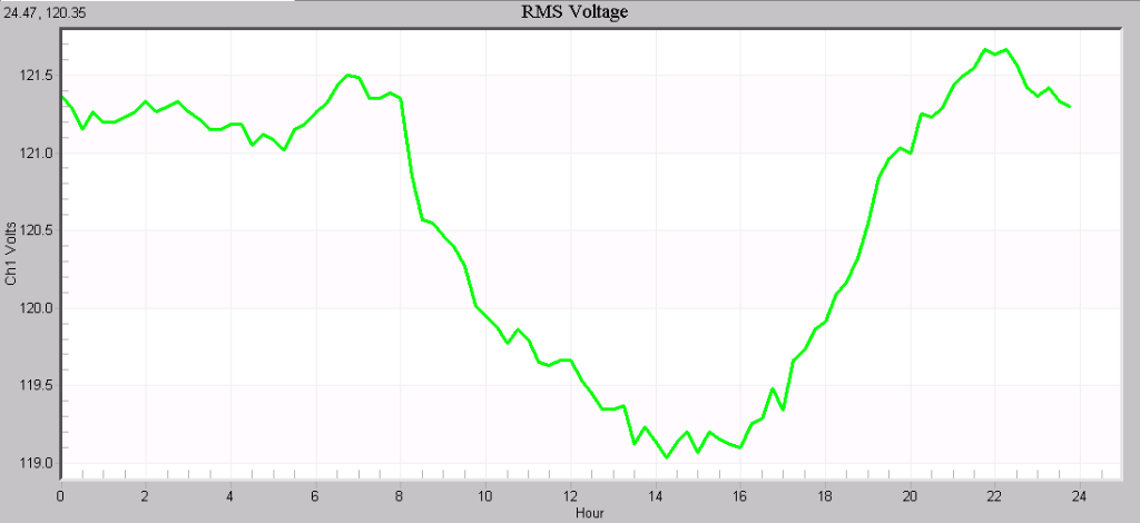
A typical RMS voltage profile is shown in Figure 1.  Here, one channel of RMS voltage is plotted.  The voltage is lowest during the day, with the minimum near 119V from 1pm to 4pm.  During early morning and late night the voltage is higher.  The highest points are 6:30am and 10pm, rising to around 121.5V.  In this example the voltage is already fairly well regulated – the swings are not that extreme.  The voltage increase near 6:30am is due to regulation anticipating the morning load increase, while the overshoot and subsequent drop in voltage near 10pm is from daily loads dropping off  (causing the voltage to rise), followed by regulation lowering the voltage.

In theory, much of the same information is available the RMS stripchart graph (Figure 2), but the level of detail here makes it difficult to isolate just the overall daily average trend.  For line regulation, the stripchart can be useful for zooming in on actual tap change events and specific operations though. 

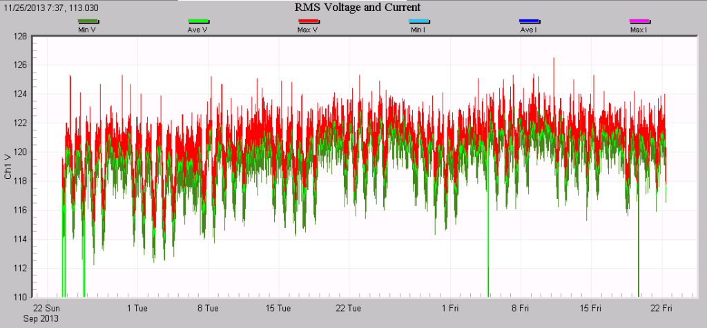
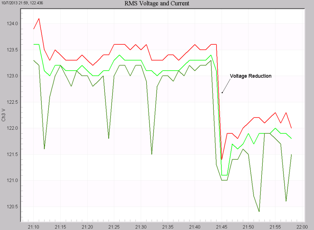
Figure 3 shows such an operation from the same data as shown in Figures 1 and 2 – a voltage reduction near 10pm.  This step change in voltage appears in the min, avg, and max traces (dark green, green, and red).  Note the voltage sags before and after the voltage reduction, which only appear in the dark green min trace.  These are averaged away in the Daily Profile, helping to separate voltage regulation trends from unrelated sags.

Local Loading

When analyzing a voltage Daily Profile, be sure to check the RMS current graph as well.  The line voltage on the transformer secondary is more heavily influenced by the secondary loads than the primary distribution voltage.  If local secondary loading is high, the voltage as measured on the transformer secondary (or worse, at the service entrance or inside a facility) may be much lower than the distribution voltage.  The transformer and wiring impedance will cause extra voltage drop, and in this case the measured secondary voltage may not be representative of the delivered voltage to other customers on other transformer secondaries.  For ideal distribution voltage profiling select a transformer with very little or no secondary load.

Figure 4 shows the voltage Daily Profile on the top graph, and RMS current on the bottom graph.  There is a clear daily trend to both, but the situation is more complex.  The current is very low from midnight (left edge of graph) until around 7:30am, so during this period the local load cannot affect the voltage too much.  In this region, the voltage daily profile is a good reflection of the primary voltage, and shows a rise in voltage from 6am until 8am.

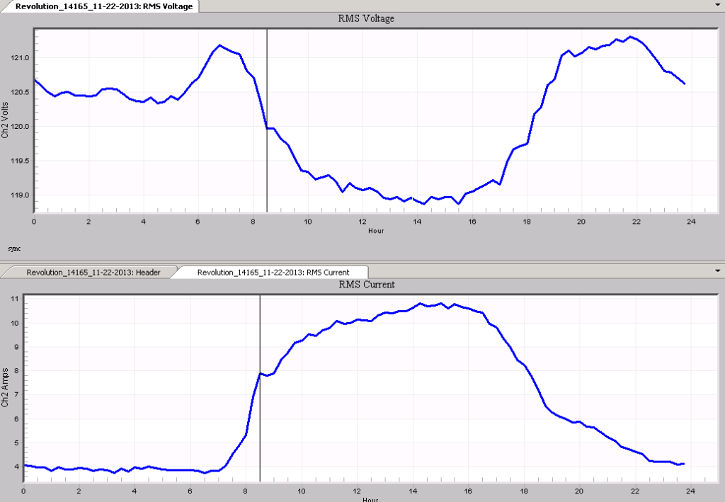
As the load increases, the voltage sags significantly. The closely matched shape of the voltage sag and current loading curves suggests that the load current is causing the sagging.  If this is the case, then the primary voltage is probably not shifting nearly as much, and other customers may not experience the same sagging.  Looking at the transformer size compared to the absolute current can help determine if the voltage sag is local or not, but in this case the graph  offers more clues.  An abrupt leveling of current around 9am is matched exactly by a leveling of the voltage sag (both marked by vertical annotations in the graph).  This mirroring is an excellent indication that the load current is mostly responsible for the voltage sag during the day.

As the current lowers towards the evening, the effect on the measured voltage is decreased.  The evening current reduction is much more gradual than the morning increase, so there is no single time where the voltage profile starts follows the distribution voltage again.  The voltage and current trends are mostly uncorrelated by 8pm; by that time the measured voltage profile is increasingly the same as the actual distribution voltage profile.

Distributed Generation

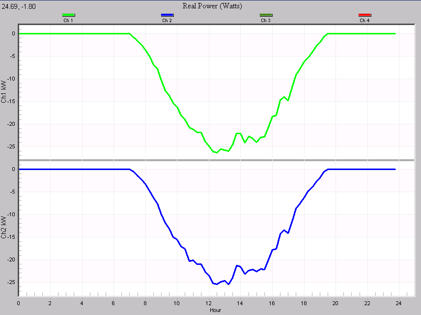
A new voltage regulation problem is introduced by distributed generation.  Here, secondary current can cause voltage swells as power is injected in to the system. In Figure 5 a single-phase location is shown with a photovoltaic system.  The top plot is the RMS voltage Daily Profile and the bottom plot is the RMS current Daily Profile.  Instead of the traditional voltage sag during the day, the voltage rises almost 4%.  This happens while the current increases from zero to 50A per channel.  The reason for this backwards relationship is shown in Figure 6: a 50 kW photovoltaic system is generating power during the day, appearing as negative power in the Daily Profile.

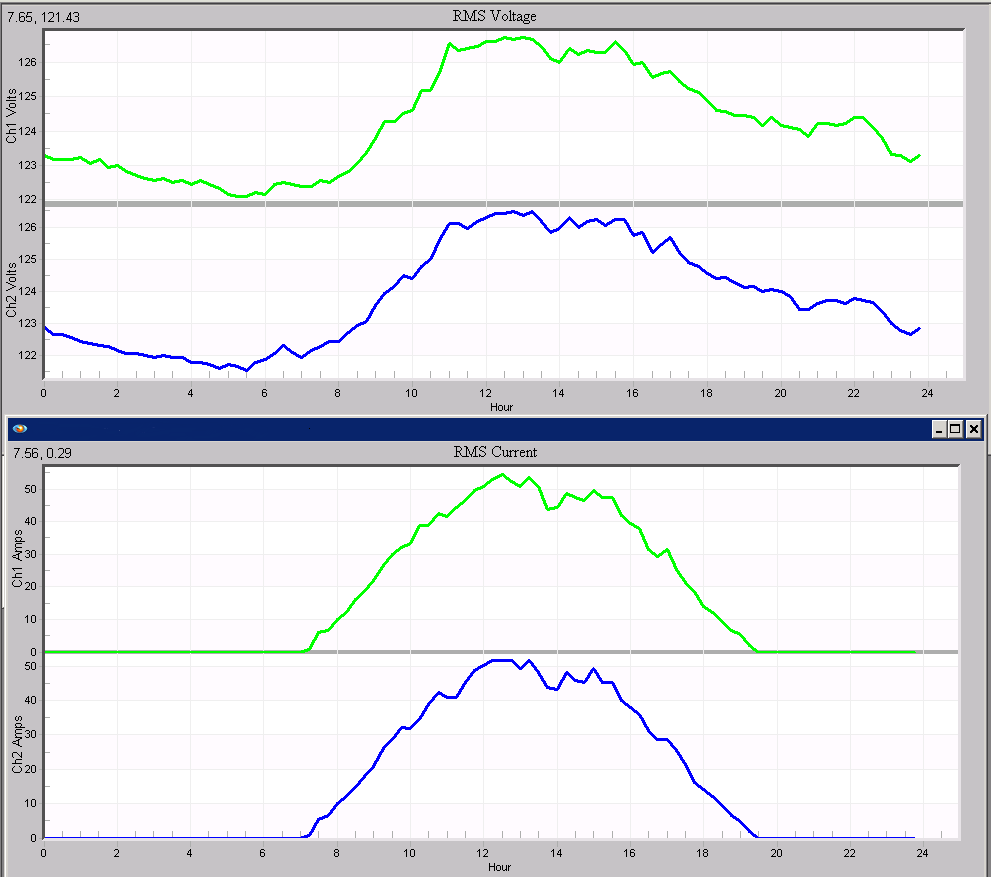
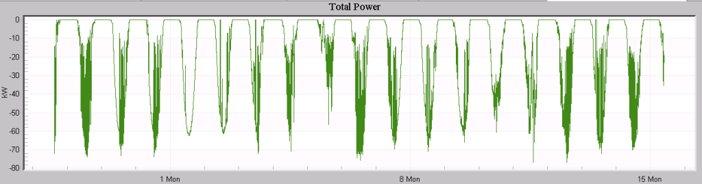
Figure 6 is another good example where the Daily Profile averaging brings out periodic trends.  Figure 7 is the total real power stripchart for the same recording.  Clearly there is a daily pattern, but each day contains significant variations due to cloud cover, local loads subtracting from PV power into the grid, etc., making it difficult to get a handle on the overall system.  The PV output timing of an “average” day is much clearer in Figure 6 than Figure 7.

Conclusion

Daily Profiles are an important graph type that helps separate 24 hour trends from extraneous one-off events.  Since many load patterns follow a 24 hour cycle, voltage regulation analysis is convenient with a daily graph type.  When using the voltage Daily Profile for regulation studies, it’s also important to check the load current to help determine if measured secondary voltage variations are actually present on the distribution side, or mostly load-induced secondary side effects.