Using Python and Jupyter Notebooks to Analyze CPOW Data

Abstract

Continuous Point on Wave (CPOW) data can be, by its very nature, exceptionally difficult to work with. The data sets can be in the hundreds of terabytes and the resolution of any segment of that data can be so fine-grained that making any sense of it at all can be overwhelming.

PMI provides both the hardware for collecting CPOW data (the Phalanx) and a high performance C-language backed Python library that seamlessly integrates with Python 3.8, Matplotlib, NumPy and SciPy all within a Jupyter Notebook environment.

This white paper showcases some of these library features, such as fault identification, recloser operation identification and some methods and tools for substation power quality analysis.

Continuous Point On Wave

Briefly stated, Continuous Point on Wave (or CPOW) data is a continuous high resolution data set of raw waveforms captured from a power system. PMI’s CPOW recorder, the Phalanx, can sample up to three channels of voltage and three channels of current on up to 12 substation feeders (for a total of 72 data feeds) concurrently and continuously. The recorded data is sampled at 256 samples per cycle, every cycle of every second of every minute of every hour of every day until disconnected.

That data is compressed and continuously streamed to an Amazon Web Services (AWS) elastic file system (EFS) data share where it is kept indefinitely.

PMI’s Jupyter Notebook analysis system also sits at Amazon and provides a read-only look into the recorded and uploaded CPOW data.

Jupyter Notebook

Jupyter Notebook is a web-based Integrated Development Environment (IDE) originally designed for big data analysis and scientific computing. The platform provides tools for rich text editing, LaTeX formatting for mathematical equations and a host of other typesetting oddities, while also providing the author the ability to inject live Python code snippets that can be evaluated repeatedly throughout a document.

These embeddable Python segments are extremely versatile. Depending on the source code, the user has the ability tocreate output in the form of static graphs (such as from Matplotlib), text tables, CSV output – anything that a standard Python interpreter can produce. Combined with the capabilities of the rich text and equation editing elements available within the Jupyter Notebook IDE an exceptional environment exists within which a very comprehensive analysis can be conducted.

PMI’S CPOW Library

The PMI CPOW library is a UNIX-based library (64-bit Linux and 64-bit FreeBSD only) that has a light-weight Python interface layered on top of it. The bulk of the computations are conducted in C in order to fully leverage the underlying hardware (especially CPU features) and to avail itself of true per-core multi-threading.

The Python segment of the library is a syntactically terse, easy-to-use and welldocumented wrapper for the underlying C libraries. It allows the user to very quickly and easily retrieve user-defined spans of raw CPOW data from the CPOW data repository and then provides utility functions for computing values such as RMS, cycle max amplitude, total harmonic distortion (THD), power factor and many other power quality measures.

Additionally, within the confines of the PMI Jupyter Notebook ecosystem, the PMI CPOW library provides users with utility functions to find faults in a data set, identify recloser operations (including identifying the type of equipment if the user provides operation times), compute symmetrical components as well as a handful of utility Matplotlib-based pre-set graphs.

A Guided Tour Through Jupyter and PMI’s CPOW Library

NOTE: If the reader would like access to a sandboxed Jupyter notebook with access to PMI’s lab testing data for evaluation, please send a message to our tech support team for a demo account.

Initializing the Notebook with Essential Imports

Most notebooks start with an import statement to include some useful third party libraries (such as NumPy for linear algebra and simple signal processing routines and Matplotlib for graphing) as well as a handful of useful standard system libraries for manipulating and managing dates and times. (Note that the data and query time formats are all UNIX time_t epoch timestamps.)

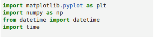
Figure 1. Common imports that are useful in most notebooks

The next imports are for PMI’s CPOW library. The native module is what provides access to the underlying C computa- tional functions. Calling enable() will load the underlying .so file and initialize the library internals. The contained_query module is a wrapper module that encapsulates all of the state necessary to perform a query for a Phalanx data set.

Figure 2. PMI library imports for analyzing CPOW data

Utility Functions and other General Setup

The next segment is a utility function that can return a tuple of start and end times. This is useful when looking through large data sets and whittling down to a specific time window for an event. The user should note that all times are in UTC.

Figure 3. A utility function for returning a tuple of start
and end time_t values. — Figure 3. A utility function for returning a tuple of start and end **time_t** values.

Querying and Graphing a Single Trace

The library is designed in such as way as to allow the user to query a single trace (a single contiguous data array corresponding to one channel of either voltage or current) or all six traces at once. The first example shows how to retrieve channel 1 voltage from the PMI lab Phalanx unit. The output returned is an instance of a wave_buffer object that exposes a handful of convenience functions that operate on the encapsulated CPOW data.

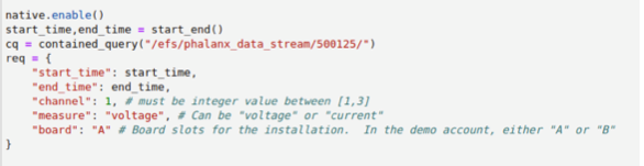
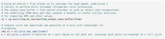
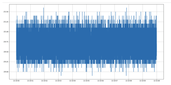
Figure 4. Creating a stand-along request object to retrieve a
singular trace of data from a Phalanx CPOW data set — Figure 4. Creating a stand-along request object to retrieve a singular trace of data from a Phalanx CPOW data set

Since the return type for that function was an instance of wave_buffer, we are able to call a couple of utility methods in order to get some quick, useful output that will allow rapid data analysis. In this particular example, we will compute the cycle_max_amplitude(). This function does exactly as it advertises: it goes cycle to cycle and takes the maximum of the absolute value of all points in each cycle and returns a singular value per cycle.

Additionally, this segment uses the wave_buffer utility method to generate an x-axis array that will be used in plotting time stamps along the X-axis of the Matplotlib graph.

Figure 5. Computing cycle max amplitudes and using a utility function
to generate a time stamp x-axis array for a Matplotlib graph — Figure 5. Computing cycle max amplitudes and using a utility function to generate a time stamp x-axis array for a Matplotlib graph

Figure 6. Output of the first Cycle Max Amplitude graph. Note that
these are instantaneous values, not RMS values. It is also worth noting
that the Phalanx is connected to a lab steady state power source. — Figure 6. Output of the first Cycle Max Amplitude graph. Note that these are instantaneous values, not RMS values. It is also worth noting that the Phalanx is connected to a lab steady state power source.

Querying and Graphing All Traces

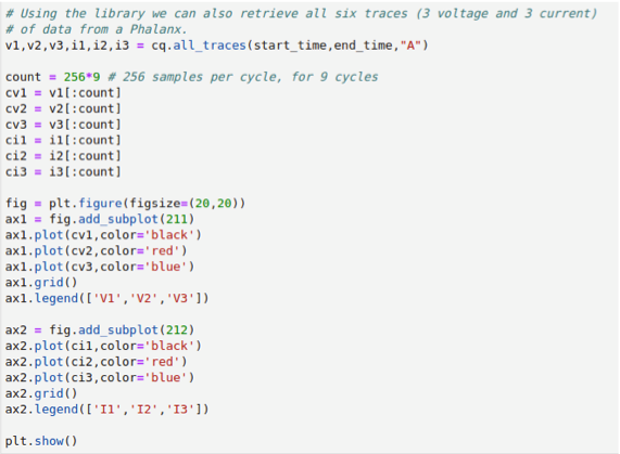
The next segment in the Jupyter notebook is an example showing how to retrieve all six traces (3 voltage and 3 current) from a single sensor board on a Phalanx. Note that there’s no explicit request dictionary passed this time – only the start time, end time and board name. The return value is a tuple of 6 wave_buffer objects (note also that the all_traces() method defaults to returning wave_buffer objects and it doesn’t have to be explicitly requested).

Figure 7. Retrieve all six traces (3 voltage and 3 current) from a
Phalanx sensor board. — Figure 7. Retrieve all six traces (3 voltage and 3 current) from a Phalanx sensor board.

Graphing Raw CPO Cycle Data

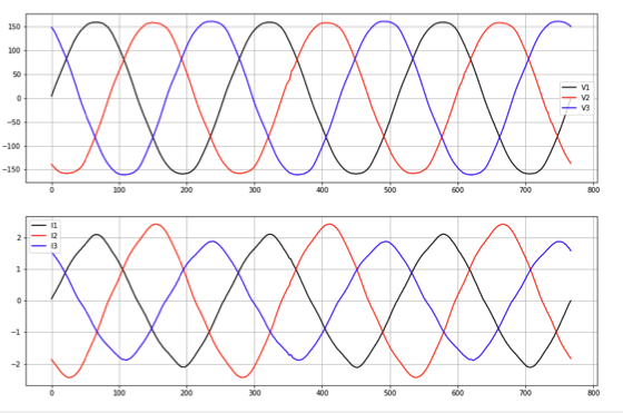
In the next segment, the first few cycles of returned data for each trace are extracted from the dataset and then graphed on two separate plots, one for voltage and one for current.

Figure 8. Raw CPOW waveforms plotted using Matplotlib

Fault Identification

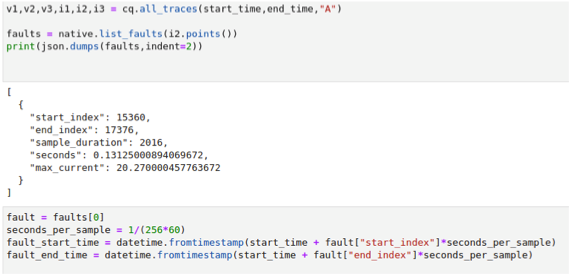
One of the more useful features of the library is its ability to take any trace of current data and identify faults within it. The output is a list of hash maps (or python dictionaries) containing useful information such as the fault duration in samples, in seconds and the max fault current. Additionally, since the fault location routine is “time unaware”, it returns the indices within the trace where the fault begins and ends. Since the start time of the trace is metadata that the caller has, identifying the actual beginning and end of a fault in time is trivial.

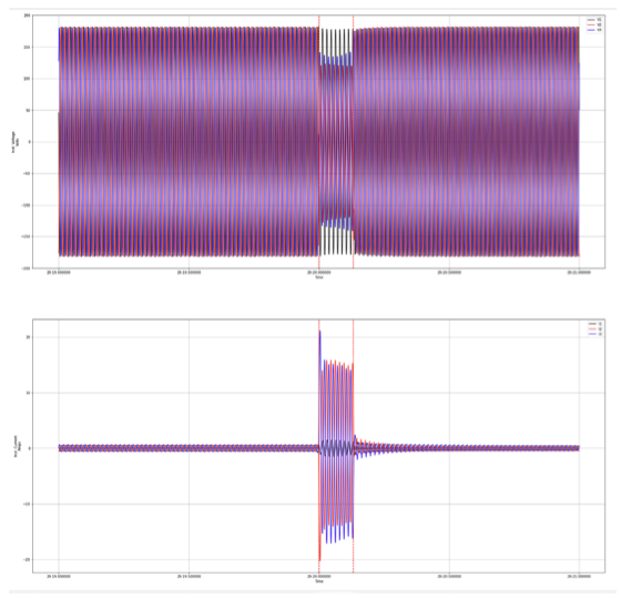
See Figure 9 for a demonstration of calling the fault identification code, a quick snippet of the fault output using a JSON output formatter, and an example of computing the fault start and end times from their given fault indices. Figure 10 is a graph of all six traces (3 voltage and 3 current) that has horizontal, dashed lines indicating the offsets of the beginning and end of the detected fault. Those are drawn at the computed fault start and end times from their indices from the previous step.

Figure 9. Fault identification and its output. Also shown: how to
compute the fault start and end times from their reported indices — Figure 9. Fault identification and its output. Also shown: how to compute the fault start and end times from their reported indices

Figure 10. Drawing a fault graph with horizontal markers to denote the
algorithm’s accuracy in detecting fault time boundaries. — Figure 10. Drawing a fault graph with horizontal markers to denote the algorithm’s accuracy in detecting fault time boundaries.

PQ Computations

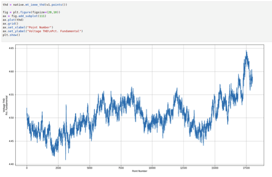
The PMI CPOW Phalanx library provides high performance functions for computing many of the standard power quality metrics desired for conducting substation power quality analysis. Examples include Voltage Unbalance (computed from symmetrical components), raw Symmetrical Component output, Total Harmonic Distortion (THD), Power Factor and others.

Figure 11. Computing Voltage THD is as simple as a one-liner
with the PMI library. — Figure 11. Computing Voltage THD is as simple as a one-liner with the PMI library.

Conclusion

Collecting, analyzing and making any practical use of CPOW data can be quite a daunting task. This white paper illustrates how PMI has laid the groundwork and provides some easy-to-use, powerful, useful and intuitive tools allowing anyone with a fundamental grasp of Python and Jupyter to create highly detailed, illustrated CPOW driven reports with little effort.