
Abstract
Parametric graphs present a little-seen view of load waveforms. By graphing the current waveform against the voltage, a voltage-independent load signature can be established. This is useful for characterizing load properties, and establishing a baseline signature for comparison with future recordings.
Parametric Graphs
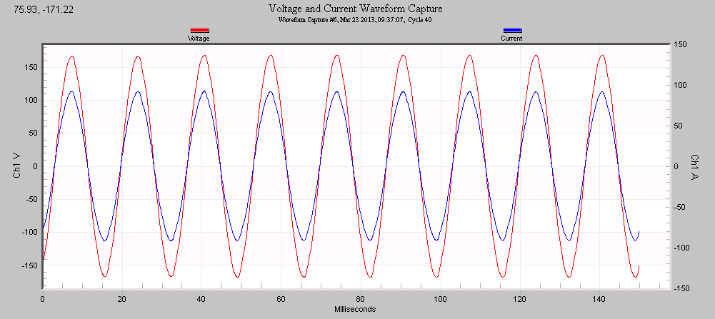
Voltage and current waveform data is most often presented as two time series, plotted with instantaneous voltage and current values on the y-axis, and time on the x-axis. Figure 1 shows the standard ProVision display. Here the voltage (red) is plotted on the left y-axis, and current (blue) on the right y-axis. The x-axis is time. The current appears to follow the voltage shape (both are relatively clean sine waves), and there is no visible phase shift. Thus, this is a resistive load.
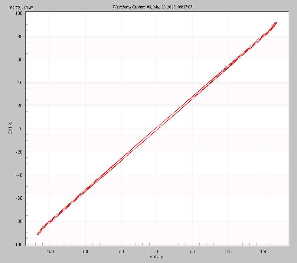
A parametric plot of the same data set appears in Figure 2. For each instantaneous voltage and current sample k, the kth voltage sample is used as the x-coordinate, and the kth current sample is the y-coordinate. The point (V[k],I[k]) is plotted on the graph, and successive points are connected with lines. The resulting graph represents the current that the load draws at each instantaneous voltage value. This parametric plot is the same type generated by an oscilloscope in “X-Y mode”, where the channel 1 input is voltage and the channel 2 input is current.
To generate this graph in ProVision, first graph any waveform capture in the normal manner (Graph, Waveform Capture, Voltage and Current in the menu). Once graphed, click the Pw icon as shown in Figure 3. It’s also possible to go directly to the parametric graph by choosing Graph, Waveform Capture, Parametric in the menu, then choosing a waveform capture, but with this method you don’t see the time series first. Without a lot of experience reading parametric graphs, it’s recommended to start with the regular waveform to ensure it’s representative of the desired load, then switch to the parametric view.

For a resistive load, Ohm’s law results in the instantaneous current being exactly proportional to the instantaneous voltage at each point, and the constant of proportionality fixed throughout the graph. This is the case in Figure 2, where the data forms a straight line, passing through (0,0) – i.e. zero volts results in zero amps. The slope of the line is rise over run, e.g. change in current over the change in voltage. From Ohm’s law, the reciprocal of the slope is the load resistance. Reading off Figure 2, the current at 150V is 80A, which gives a resistance of 150V/80A = 1.875 Ohms. Any other points on the line give the same 1.875 Ohms, since the slope is constant throughout the waveform. The more vertical the line, the lower the load resistance. A horizontal line (passing through the origin) would be infinite resistance – that is, an open circuit. A near-vertical line would be a dead short, with the current limited only by the network wiring.
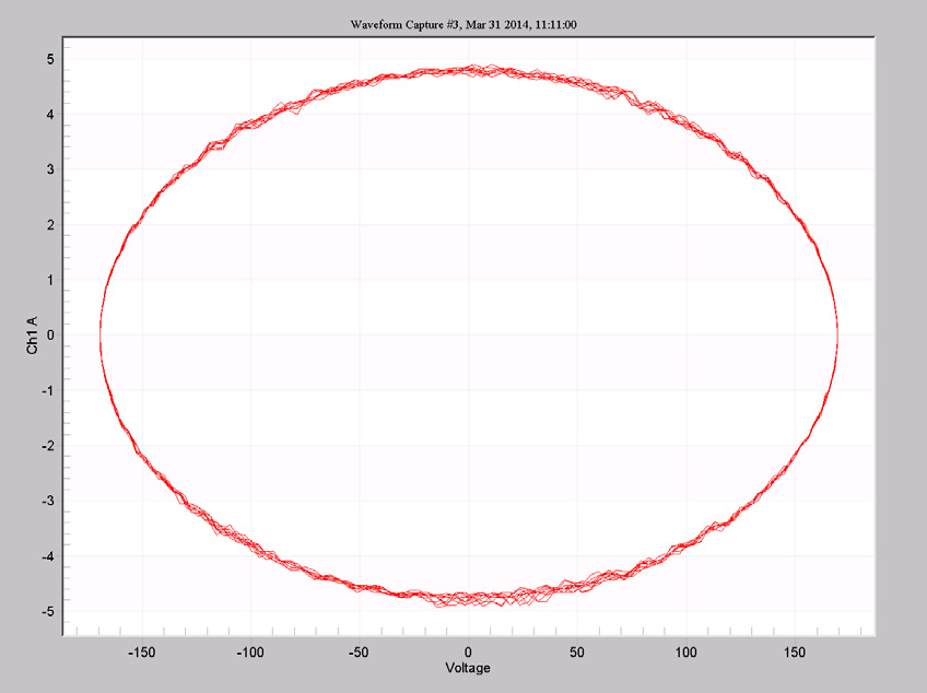
A reactive load will produce an ellipsoid pattern, due to the phase shift between voltage and current. The greater the phase shift, the closer the ellipsoid approaches a circle. With a full 90 degree phase shift (either purely inductive or capacitive), the graph will be a full circle. The narrower the ellipse, the smaller the phase shift, with the limiting case of a straight line for no phase shift. A pure capacitive load is shown in Figure 4. For any given ellipse shape, the more vertical the long axis, the lower the load impedance, as with the resistive case. The parametric plot with a linear load (resistive plus some reactive component) is a special case of the more general Lissajous curve, with the two inputs (voltage and current) at the same frequency.
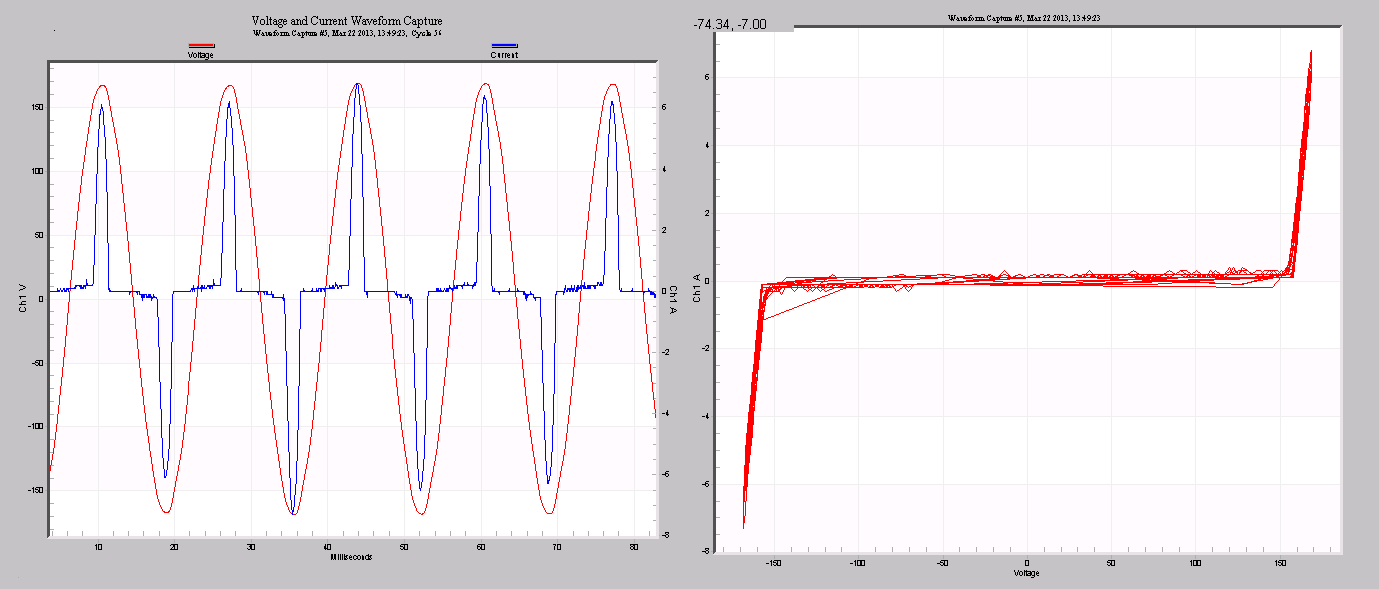
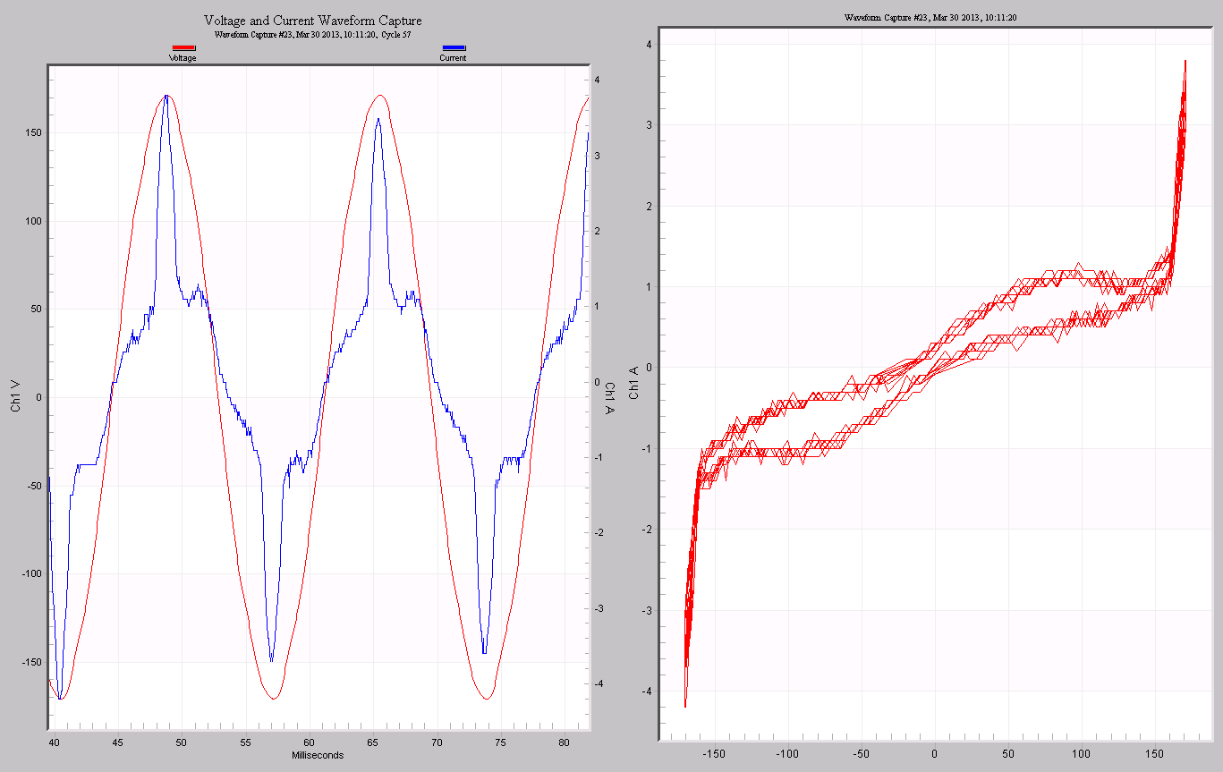
The plots become more interesting with nonlinear loads. A typical electronic load is shown in Figure 5, with the traditional and parametric plots. This switching power supply only draws current during a small conduction angle near the peak of the waveform. This property is expressed in the parametric view by the horizontal section – the region with no current flow, surrounded on each end by steep vertical lines – the region of large current flow. The slope of the two vertical lines is the same, and represents the load impedance while current is allowed to conduct.
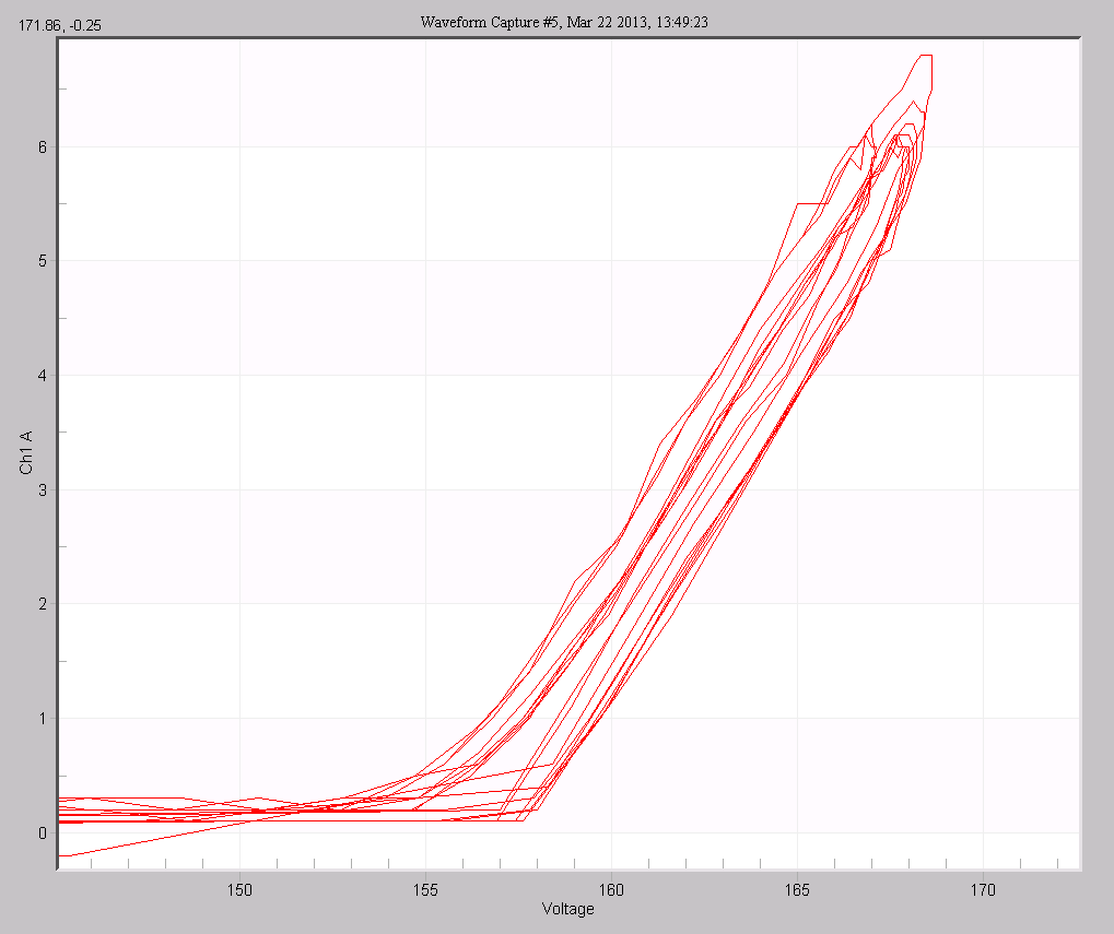
Zooming in on the left section (Figure 6) reveals that there is a reactive component to the current flow, but it’s mostly resistive (the width of the ellipse is very small compared to the length). Reading off the graph gives an estimated load resistance of 166V/6A = 27.5 Ohms. The multiple loops in the figure are the multiple cycles in the waveform capture – each complete 60Hz cycle is a complete excursion from the negative to positive voltage extreme, and another loop through the parametric graph. If the load characteristic is identical each cycle, those loops will be identical, and the graph will look as if only one were plotted. In most cases (especially if the waveform was triggered by a load change), the load changes slightly from cycle to cycle, producing closely spaced loops.
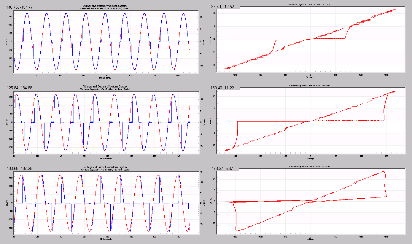
An SCR switched load is shown in Figure 7, with three different switching points. The general shape of the parametric plots is a “bow-tie.” In the top plots, the SCR is conducting most of the time, and the parametric plot is mostly a straight line (indicating a resistive load). The small bow-tie in the middle formed by the horizontal line is the portion where the SCR is off, and thus no current is flowing (y-axis values all zero). Although the “off” portions are very small in terms of time, the voltage sine wave goes from 0 to 70V, and down from 0 to -70V during those portions. The slope of the sine is highest at zero crossing – here the voltage changes very rapidly vs. time, and so any current activity (or non-activity) is magnified on the x-axis in the parametric plot. In the middle and bottom plots, the SCR off time is increased further, and the bow-tie portion in the parametric plots grows larger and larger.
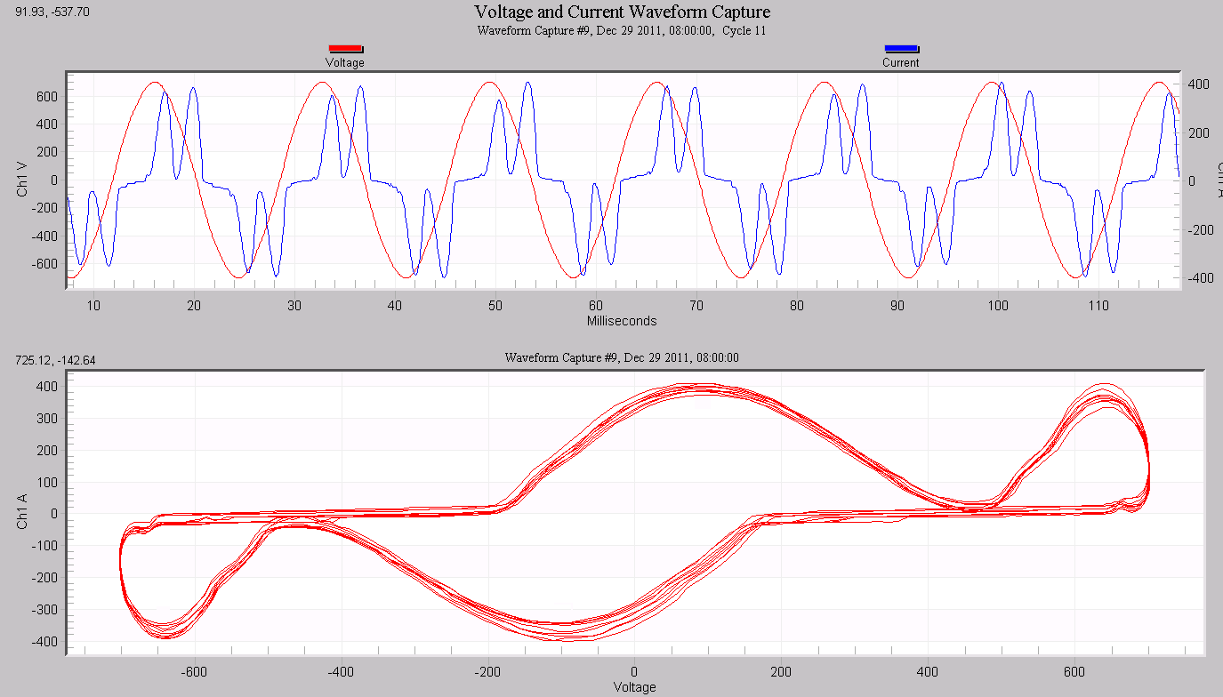
A 6 pulse converter, the typical front-end for a variable frequency drive, is shown in Figure 8. In a single phase, there are four current pulses that repeat each cycle, and these appear as lumps in the parametric plot. The four pulses are labeled A, B, C, and D on each graph to show the correspondence between the two views. Although the pulses are approximately the same time duration, pulses A and C are narrower than B and D in the parametric plot, since they span a larger range of voltage values in the sine wave. Again, the sine wave changes values much faster near zero crossing (i.e. the slope is greater), thus for a given fixed time width, the voltage values at the start and end time will be further apart there as compared to the region around the waveform peak.
The full 3 phase plot in Figure 9 shows that the current pulses are not quite balanced, especially in channel 2 (middle plot). This is visible in the parametric plot for channel 2 – the “B” lump has a lower amplitude than the “A” lump.
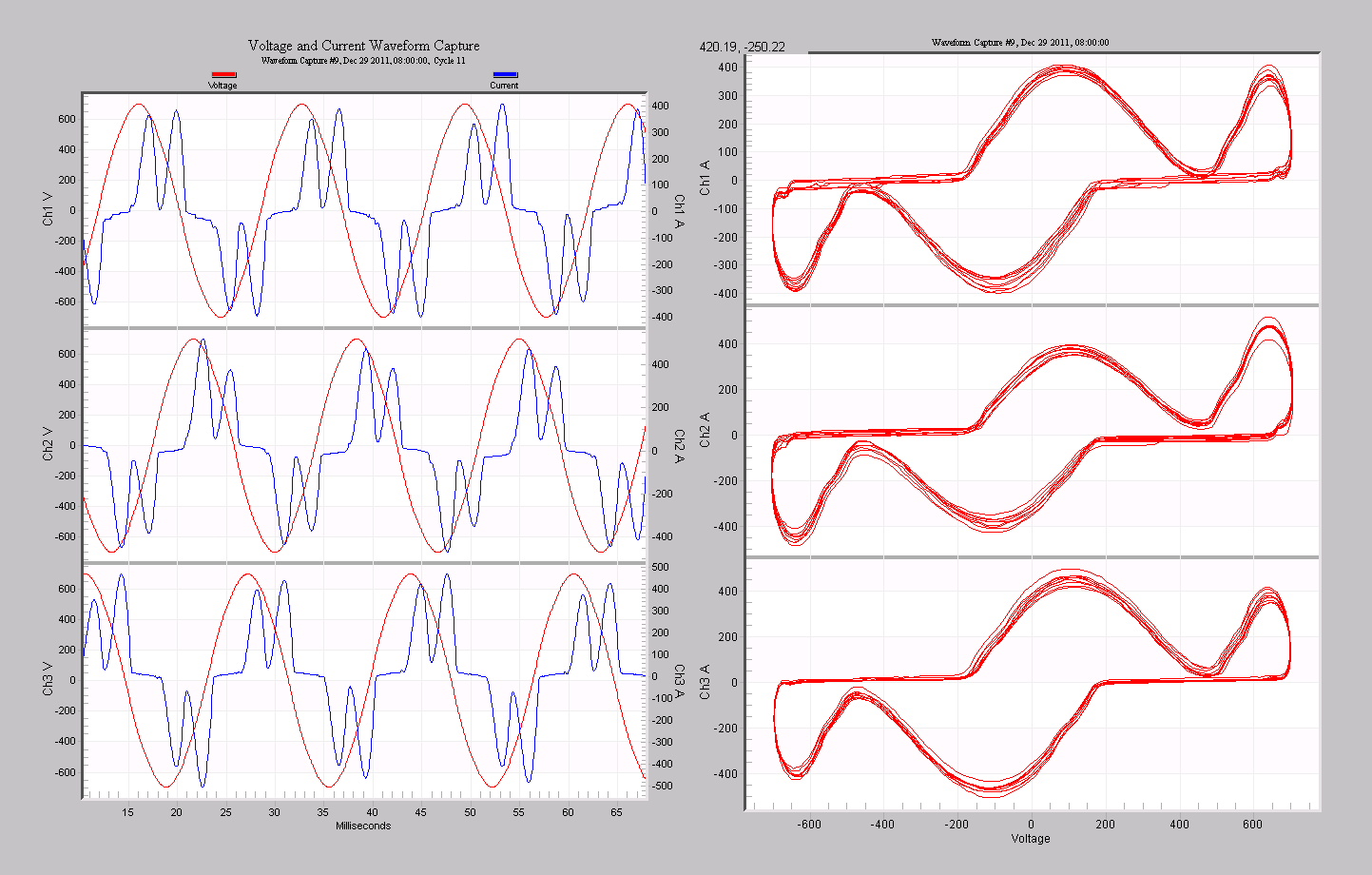
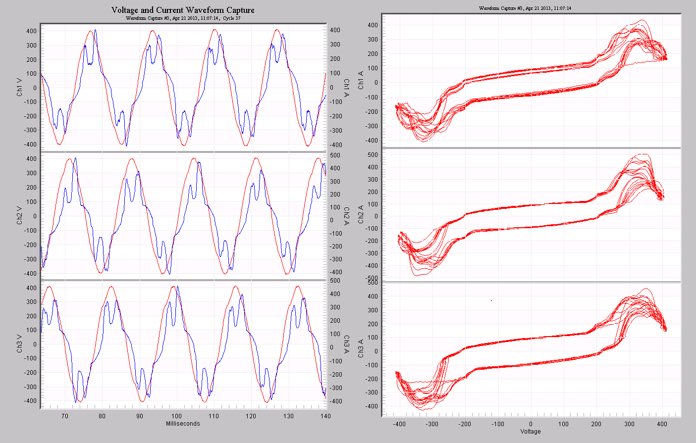
A mix of load types will produce a more complex parametric graph. In Figure 10, a mix of mostly switching power supplies, along with some 6-pulse converter load is shown. The 6-pulse lumps are visible, but much smaller than the current spikes at the ends of the parametric plot. In Figure 11, a 3-phase mix of “6-pulse”, linear, and other more unusual nonlinear patterns are seen. In the parametric version, the V-I plots show an ellipse (appearing more rectangular than elliptical) for the linear portion (not purely resistive, as evidenced by the vertical separation in the ellipse). The two ends of the parametric plot show the more nonlinear behavior. The “B” and “D” lumps from the earlier 6-pulse converter plot are missing here, due to the different phase shifts with the pulses in this capture. The pulses here were not produced by a simple 3-phase bridge rectifier, and produce a much different parametric plot.
Parametric graphs give some interesting views, but how are they used? These plots are most useful when a single load is monitored. They give a voltage-independent display of the load characteristic – the parametric plot, in theory, should be unchanged if the voltage waveform changes. At the very least, it’s less sensitive than the standard time series display. These load signatures are useful for troubleshooting large loads such as simple AC and VFD-based motors. Reference parametric plots should be stored during “normal” operation, for comparison with later recordings to help predict failure, or troubleshoot a problem. For equipment manufacturers, the parametric plot reveals characteristics about the load that are not as easy to spot in the standard waveform, such as impedance vs. point on waveform. In a collaborative troubleshooting process, these graphs can be shared with the customer or equipment manufacturer to help determine a root cause.
For monitoring of aggregate loads (e.g. at service entrance, substation, etc.), the parametric plots allow for an easier determination of load impedance. Impedance can be estimated on a regular waveform capture graph by picking a point on the voltage and current sine waves (at the same time), and dividing, but a more accurate estimate is possible by using the parametric graph, and using the slope of a linear portion. The vector diagram can also be used for impedance calculations, by dividing the voltage and current phasors, but this assumes a constant impedance throughout the waveform, and ignores harmonics.
Conclusion
Parametric graphs are a less common method of viewing waveforms, but can reveal details not obvious in standard time-series displays. They are especially useful when monitoring specific complex loads, and can be compared to reference signature plots to reveal changes in the equipment, or problems.