
Abstract
Ensuring that service voltage is within ANSI limits is a basic but important step in delivering power. Sophisticated programs such as Conservation Voltage Reduction (CVR) and volt/VAR optimization require continuous steady-state monitoring as switch operations are made by the system. These steady-state voltage measurements should include the effects of voltage sags and other short-term excursions. On the other hand, a fast response and near real-time readings are needed for immediate feedback for automatic systems.
It was for these very purposes that PMI designed the Boomerang monitor and the Canvass web application. The Boomerang is a permanent monitor that constantly provides 1-second RMS voltage (and on select devices current and real power) readings to Canvass. These readings may be viewed with an adjustable, sliding averaging window for “what-if” and engineering analyses of system voltage all through the distribution network.
This whitepaper discusses how to use Canvass and Boomerang to perform longer-term trend analysis for CVR and for basic system profiling by adjusting the averaging interval (increasing it from the standard 1-second interval to a user-defined value) and observing the results graphically.
Calculating the Averaging Interval
It is useful to begin by describing the averaging algorithm used by Canvass when rescaling the data based on a user-provided interval.
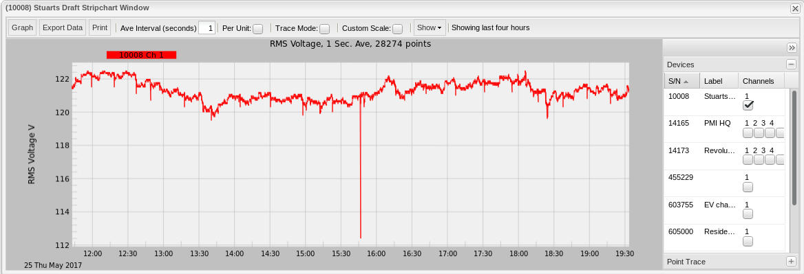
When no custom-interval is specified, the graph contains all of the points as reported by the device with its 1-second averaging interval. This provides a relatively high-resolution view of the voltage (or current or real power) data and can be exceptionally useful for finding very short-duration sags and swells over a given period of time. Figure 1 below demonstrates a stripchart graph at a default 1-second interval.
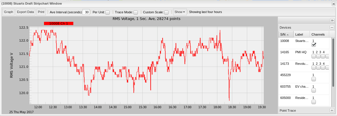
Sometimes, however, this fast response time isn’t necessary or is even counter-productive. In these scenarios, a wider averaging window can be employed to “smooth out” the shape of the graph. Figure 2 shows the exact same data as Figure 1 but averaged at a 30-second interval. Note the sag at 15:45 is no longer there. This is a result of the averaging algorithm.
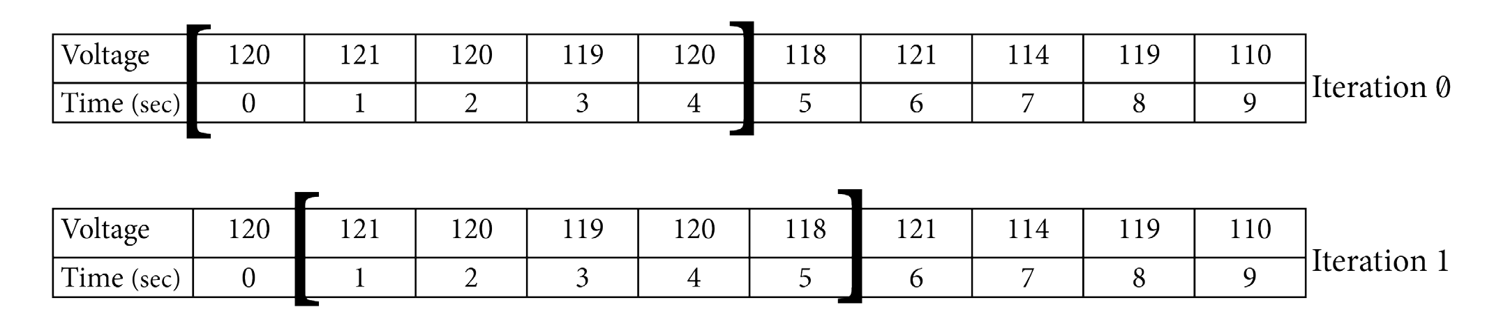
The averaging algorithm is implemented as a “sliding window” average, to maximize response time and reduce artifacts. Instead of taking 30 points (for a 30-second averaging interval) and reducing it to 1 point (thus reducing the data in the graph by a factor of 1/30), the algorithm starts at point 0, then averages the next 30 points into a new value and replaces point 0 with the new average.
It proceeds to point 1 and picks the next 30 points, averages them and replaces point 1 with that value. That continues for each point in the graph (except for the final points, where any remaining length < 30 is averaged into the remaining point). For example, if the averaging interval is 30 seconds and the sliding index has reached point 25 of 30, then that point is the average of the remaining 5 points, not the remaining 5 and an additional (but not graphed) 25. Figure 3 is a graphical representation of how the algorithm works.
The sliding nature of the window gives 1-second time resolution even with a longer averaging interval. An alternative method is to move the window an entire averaging width at a time (e.g. with a 5-minute window, the window jumps 5 minutes at a time). This method produces artifacts at the edges of the interval when it jumps from one value to another. It also reduces the time resolution to the interval length instead of the raw 1-second time stamp.
Specifying an Averaging Interval
The averaging interval must be specified in seconds (as noted in Figure 3). Common custom averaging intervals are:
- 30 seconds
- 60 seconds (one minute)
- 300 seconds (five minutes)
- 600 seconds (ten minutes)
- 900 seconds (fifteen minutes)
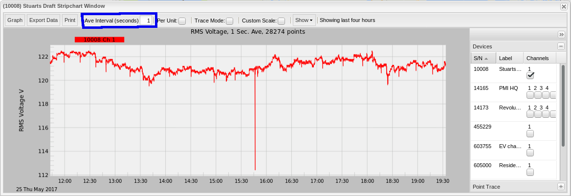
The current Canvass implementation does not allow an averaging interval beyond 15-minutes (900 seconds). Once an averaging interval is specified by typing the number of seconds into the “Averaging Interval” text box (Figure 4), simply click the “Graph” button to the left of the averaging interval input.
Selecting an Averaging Interval
While changing the Averaging Interval for the graph is quite simple, selecting which interval to use requires a little bit more thought. A small averaging window and the voltage will react too quickly to relatively short sags or swells; a window that is too large and the system may be too sluggish to react to moderately large events.
ANSI limits are often defined around a 5 or 15-minute average. It’s helpful to examine the system voltage with the official utility-defined standard to ensure that each monitoring point is in compliance.
An analysis with a smaller interval, such as 1 or 2 minutes, is very useful for spotting faster changes during tap changes or switching events. In general, a shorter interval can shed light on the underlying movements behind the “official” 5 or 15-minute average.
Figure 5 shows a Boomerang at a 120V nominal. Note the frequent local voltage sags, which are unrelated to steady-state system voltage regulation. These sags are likely only present on the transformer secondary. These sags are relatively frequent, but also very short in duration.
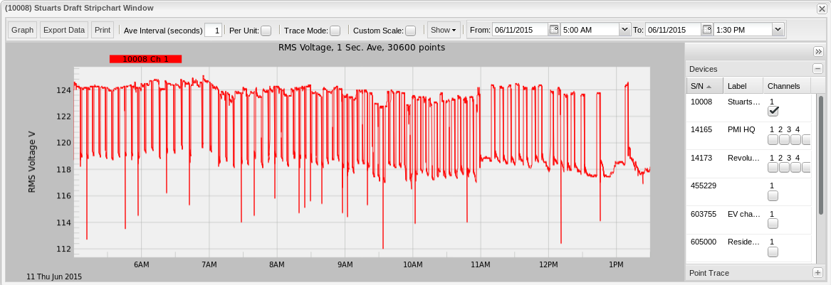
Figure 6 shows the exact same data but averaged at a one minute (60 second) interval.
Note how, while there are still several sags on the graph, all of the dips to and below 116V have now been “averaged out.” While this is better, it’s still not ideal – our continuous range from 117V to 124V is within +/- 5% but may be better without the frequent distortions. This averaging length is still too short to feed directly into a CVR system – it may respond to these local sags.
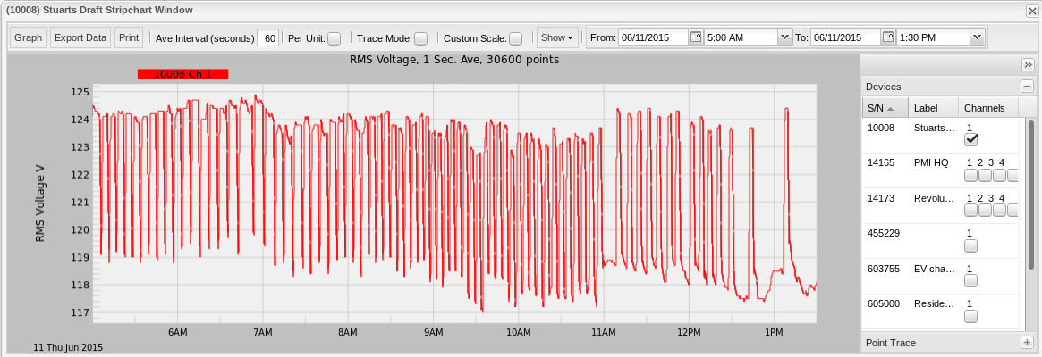
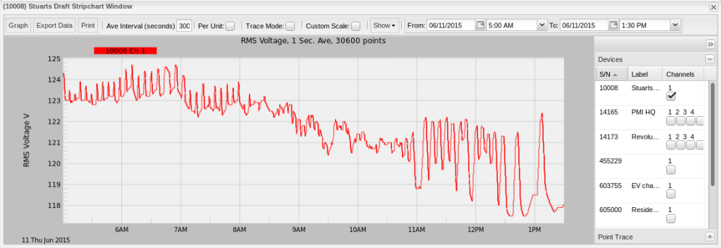
Figure 7 shows the same data re-averaged to a 5-minute (300 second) interval. Note how now all of the sags below 117V have disappeared and the wild variance from 118V to 124V has been essentially reduced to 123V to 124V (toward the beginning of the selected period).
On a 5-minute basis, the voltage regulation here is good. This window size is a better choice for automatic adjustment. With a suitable window length determined, this value may be programmed directly into Boomerangs for SCADA polling in an automated system.
Conclusion
Using Canvass to analyze steady-state voltage is quite easy. The sliding averaging window essentially removes local voltage sags and swells, while preserving 1-second time resolution. Use different window lengths in Canvass to analyze distribution voltage with respect to ANSI compliance and to track how regulators are responding.
The optimal window to use for automatic CVR or volt/VAR programs is long enough to prevent responses to short sags, while short enough to respond to true swings in distribution loads or upstream events. This whitepaper has demonstrated how to adjust the averaging interval and analyze the resulting output.