Power Theory in Multiphase Distorted Systems

Introduction

“Geometric Foundations of Power Theory for Multiphase AC systems in the Frequency Domain” is a great research article written by Francisco Montoya and others and it clearly explains a method for analyzing the power components in a distorted multiphase AC system that is not necessarily balanced. This method relies on harmonic analysis, geometric algebra, and symmetrical components to build up a general mathematical extension to the power triangle that works in any situation.  This method is important because it provides both an accurate general overview of things like power delivered vs power reflected as well as the detailed granularity that engineers need to design specific filters and compensators to mitigate particular problems. The goal of this paper is to take a real distorted 3 phase waveform and work through the multivector computations proposed in Montoya’s paper explaining any relevant concepts as they come up. 

Waveform Data

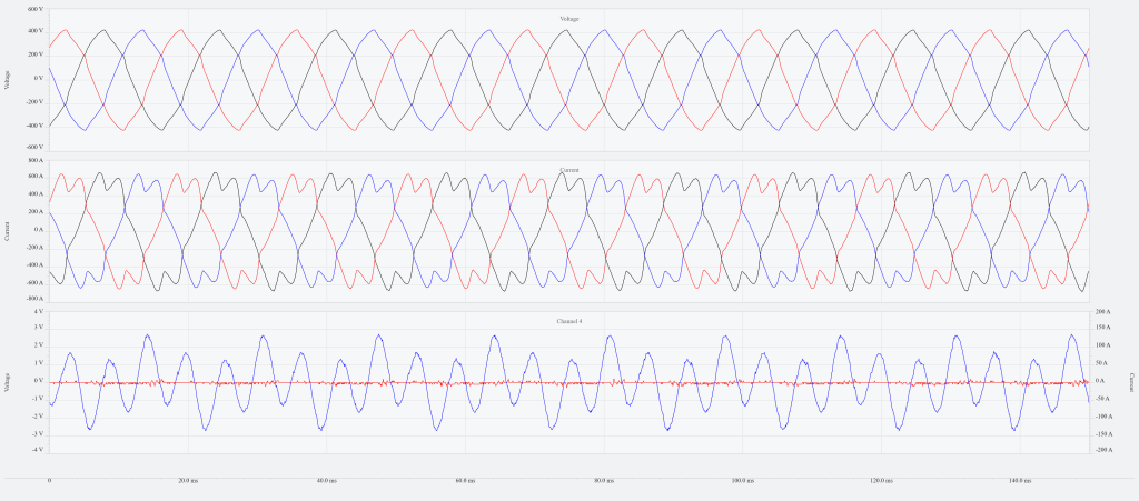
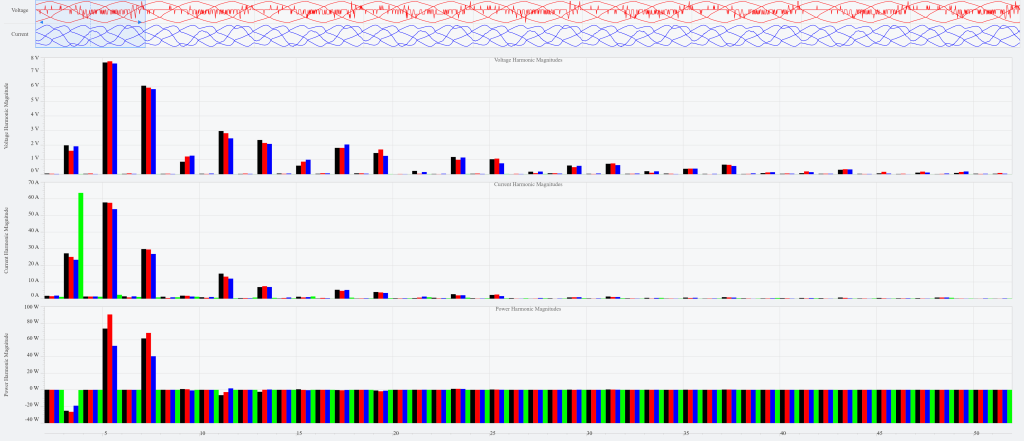
Figure 1 shows a PQ Canvass time series graph for 3 phases of voltage and current as well as an additional channel for neutral.  The dips in the peaks of the current waveform are
characteristic of a 3 phase rectification circuit with 6 diodes such as what is in the initial stage of a Variable Frequency Drive. The neutral current shows a very obvious 3rd harmonic influence, which comes from the fact that the 3rd harmonic distortion on each phase adds constructively with each other rather than canceling each other out. Figure 2 shows the PQ Canvass graph of the magnitude of each harmonic during the first cycle of the data.  

Step 1: Harmonic Components

The first step is to decompose the data signals into their harmonic components. Because the data signals are stored as 256 samples per cycle, it is useful to think of a cycle of data points running from index n=0 up to index n=255 and to construct a sequence basis around that. In this case, it turns out that the right sequence basis is given by 

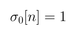
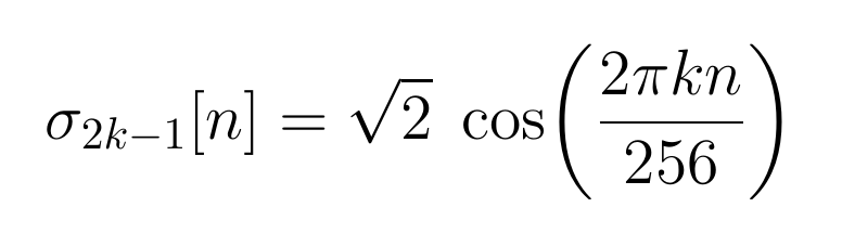
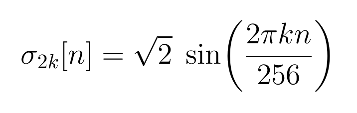
where  = 1,2,3,… upk to however high the harmonic number is relevant to be considered. Note that due to the Nyquist Sampling theorem, there is an upper limit of k=127. Sequences in this space are endowed with the inner product given by

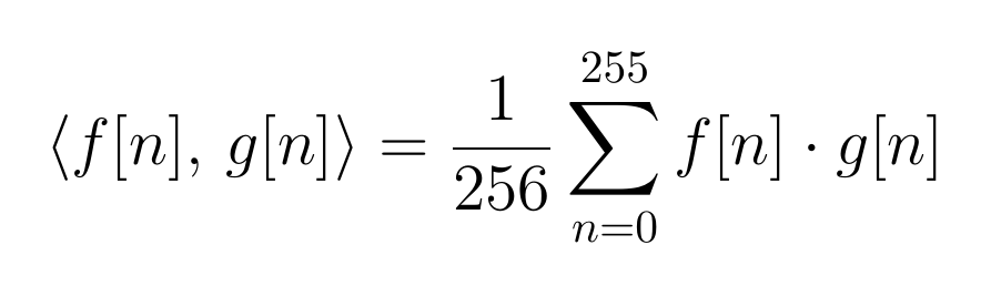
The reason why this particular sequence basis was chosen is because

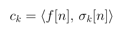
which is a much easier formula to calculate than if the basis sequences were not orthonormal. Figure 3 shows a portion of an excel sheet used to calculate these C_k  coefficients. 

Marker A is the k number that selects the particular σ_k. Marker B shows the first few rows of the raw voltage and current data readings that extends all the way to row 2308. Marker C is the computation of Θ, and Marker D is σ_k[n]which is either all 1 or or  Marker E shows the product of the raw data points with σ_k[n]. Marker F sums each of the 9 cycles in block E and divides by 256. Lastly marker G takes the average of the 9 entries in each column in block F. This shows the computation of c₁ for each of the voltage ranges and current ranges. Using Excel’s data table feature this same computation is repeated from k=0 to k=102 to get up to the 51st harmonic.  

Most of the entries in the table contribute almost nothing to the variation in the signal, so to limit unnecessary clutter in future computations, it was decided to only include harmonics if its magnitude rose above 0.5% of the nominal value.  If it fell below that threshold, then it would be ignored. Figure 4 shows the result of this filtering for voltage and current channels 1,2, and 3.

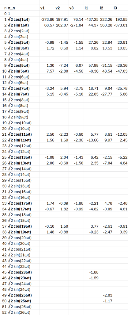
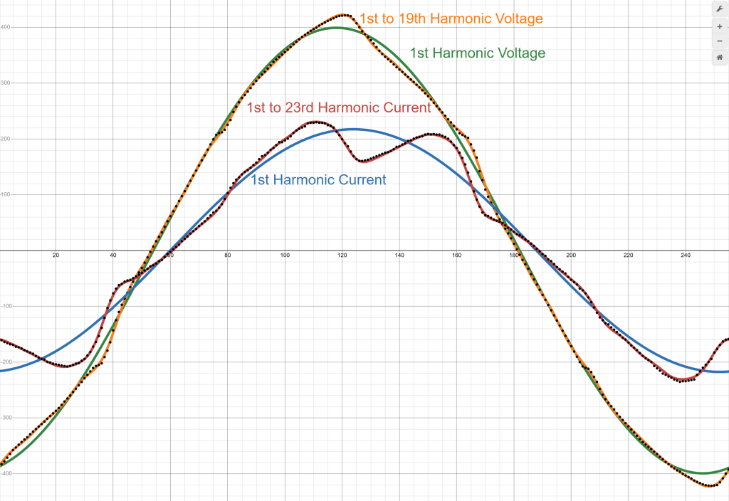
Figure 5 shows the first harmonic and all harmonics from figure 4 put together for voltage and current channel 1 as well as the individual data points showing that the calculated coefficients do describe the data points pretty well. In this graph the current scaled down by a factor of 0.4 in order to fit neatly on the plot. Channels 2 and 3 would show similar information just phase shifted by about a third of a cycle. 

Step 2: Power Analysis on Each Phase

From Figure 4, we can define the vector $\vec{V_1}$and $\vec{I_1}$ as 

$\vec{V_1} = -273.86 \sigma_1 + 68.57 \sigma_2 – 0.99 \sigma_5 + \cdots + 1.48 \sigma_{38}$

$\vec{I_1} = -437.25 \sigma_1 + 44.37 \sigma_2 + 27.26 \sigma_5 + \cdots -1.59 \sigma_{46}$

Now define

$M_1 = \vec{V_1} \vec{I_1} = (-273.86)(-437.25) \sigma_1 \sigma_1 + (-273.86)(44.37)\sigma_1 \sigma_2 + \cdots + (1.48)(-1.59) \sigma_{38}\sigma_{46}$

where the product distributes over addition and constants can be factored out. The only difference from ordinary multiplication is that commutativity is not assumed, so σ_iσ_j≠σ_jσ_i.With the 16 terms in $\vec{V_1}$ and the 18 terms in $\vec{I_1}$, there would be 288 total terms in M₁. 

The defining property of a geometric algebra or Clifford algebra on a vector space V with an associated inner product is that for any v in the vector space V, vv = v $\star$ v. This means that all the σ_iσ_i terms in M₁ can be replaced by $\langle \sigma_i, \sigma_i \rangle = 1$ This property also means that given some sum $\vec{a} + \vec{b}$, then

$(\vec{a} + \vec{b})(\vec{a} + \vec{b}) =(\vec{a} + \vec{b})\star(\vec{a} + \vec{b})$

$\vec{a}\vec{a} + \vec{a}\vec{b} + \vec{b}\vec{a} + \vec{b}\vec{b} =\vec{a}\star \vec{a} +2 \vec{a}\star \vec{b}+ \vec{b}\star\vec{b}$

$\vec{a}\vec{b} + \vec{b}\vec{a}=2 \vec{a}\star \vec{b}$

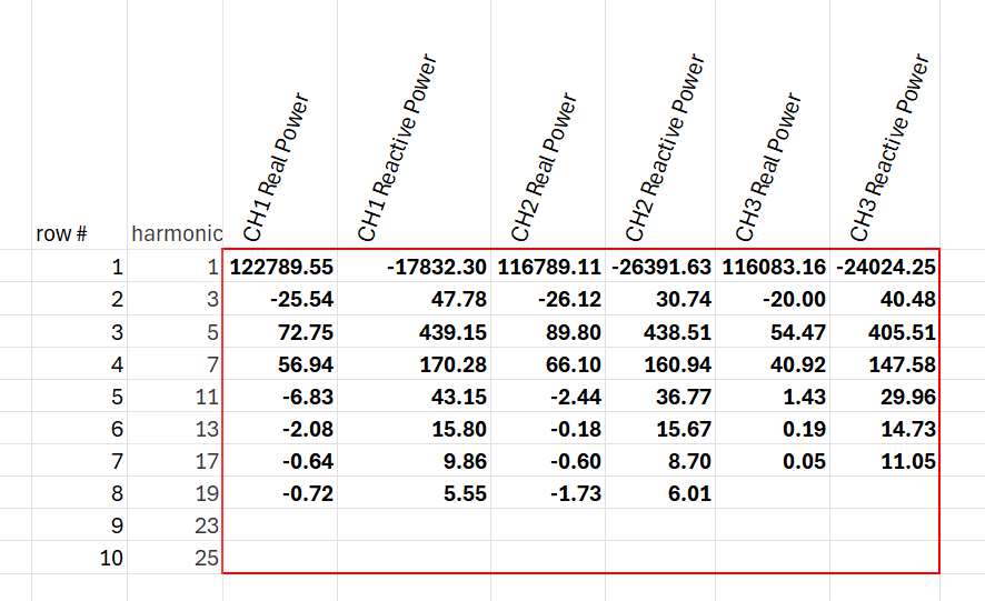
If $\vec{a}$ and $\vec{b}$are perpendicular, then $\vec{a}\star \vec{b} =0$ and the product between the vectors is antisymmetric, i.e. $\vec{a}\vec{b} = – \vec{b}\vec{a}$.  If $i \neq j$, then $\langle \sigma_i, \sigma_j \rangle =0$ by construction, implying that $\sigma_i\sigma_j = – \sigma_j\sigma_i$.  It is instructive to break off the single frequency terms as a separate piece of $M_1$ because those real parts and reactive parts correspond most directly to the traditional power triangle interpretation where the analysis is applied to each frequency.  As an example the pure third harmonic part of $M_1$ is 

$-26.95 \sigma_5 \sigma_5 – 0.81 \sigma_5 \sigma 6 + 46.97 \sigma_6\sigma_5 + 1.42 \sigma_6\sigma_6 = (-26.95 + 1.42)  + (46.97 +0.81) \sigma_6\sigma_5 = -25.54 W + 47.78 \sigma_6\sigma_5 VAR$  

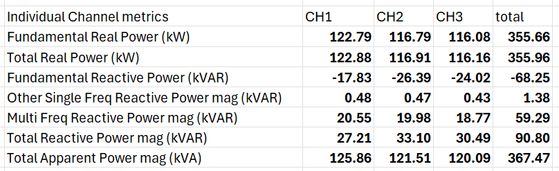
Figure 6 shows a table containing these pure frequency real and reactive components for each phase.    The rest of the terms of $M_1$ contain 144 bivector terms that correspond to a distortion power effect of applying voltage at one frequency and measuring the reflected current at another frequency.  These 144 bivector terms can be aggregated together into a single magnitude by taking the square root of the sum of the squares, which yields roughly 20.55 kVAR.  Figure 7 shows a table containing various aggregation metrics for each channel.

Step 3: Symmetrical Components 

The other important idea in Montoya’s paper is that of including symmetrical components in the analysis of
multiphase systems. The calculations in step 2 treated each of the three channels as separate isolated systems, but that is not necessarily the case. It could be that voltage on one phase induces some current on a different phase and different frequency and that contribution would not be captured in the previous step. The method of Symmetrical Components is a way to express some collection of three sinusoidal signals as a linear combination of simpler balanced sinusoidal signals.  Balanced three phase systems have all sinusoids at the same amplitude and phase shifted by a multiple of 120 degrees and are much easier to consider than the unbalanced case. The transformation to this special basis, which has the names positive sequence, negative sequence, and zero sequence, can be defined as 

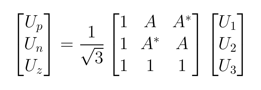
with the inverse transformation given by

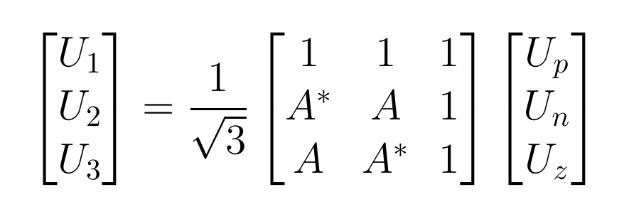
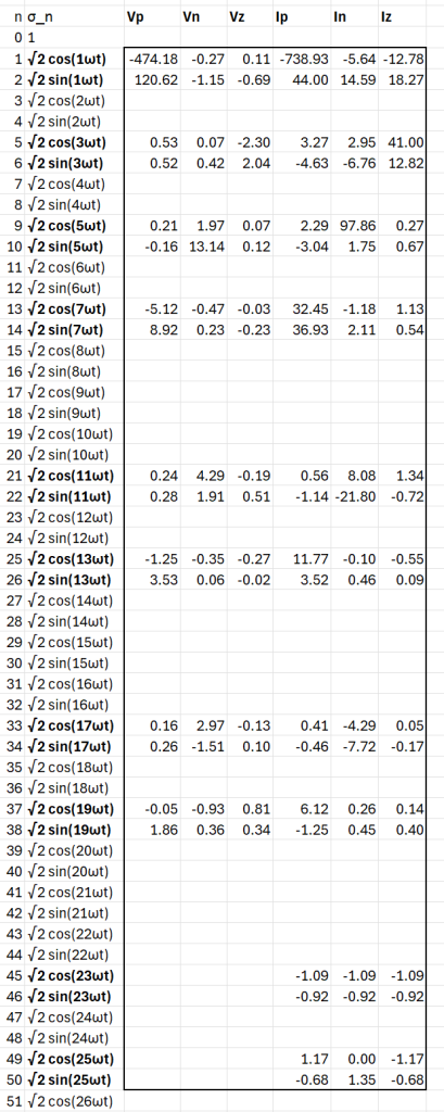
where U₁, U₂, U₃ are the individual signal phasors, U_p, U_n, U_z are the positive, negative, and zero sequence phasors, and A and A^*are the opposite rotation phasors by 120 degrees.  Switching the roles of A and A^*simply switches the positive and negative sequences. Montoya proposes in his paper to perform this symmetrical components computation on each harmonic in the voltage and current signals and then form a large vector whose basis vectors consist of the cosine and sine terms of the positive sequence coefficients, then cosine and sine terms of the negative sequence coefficients, then cosine and sine terms of the zero sequence coefficients. Figure 8 shows the result of this calculation of the symmetrical components coefficients for Voltage and Current. Note that the polarity of A was chosen to make the nominal frequency positive sequence dominate the expression, instead of the negative sequence.  We can now form the larger voltage vector as

$V = -474.18 \sigma_1 + 120.62 \sigma_2 + \cdots 1.86 \sigma_{38} – 0.27 \sigma_{51} – 1.15 \sigma_{52} + \cdots + 0.36 \sigma_{88} + 0.11 \sigma_{101} – 0.69 \sigma_{102} + \cdots + 0.34\sigma_{138}$

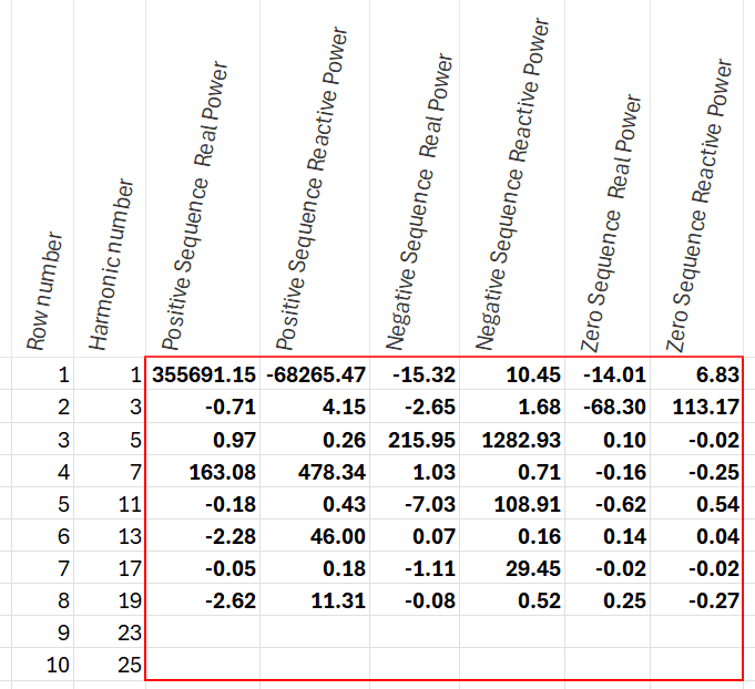
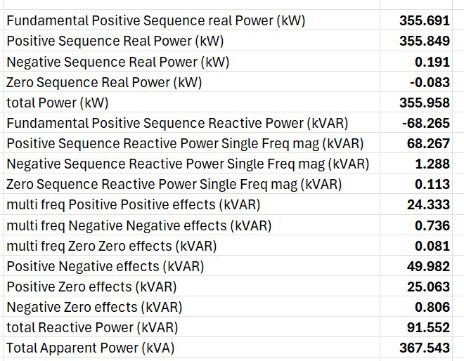
with 48 total terms, where σ₁ through σ₅₀ cover up to 25th harmonic in the positive sequence, σ₅₁ through σ₁₀₀ cover up to the 25th harmonic in the negative sequence, and σ₁₀₁through σ₁₅₀ cover up to the 25th harmonic in the zero sequence. The larger current vector can be defined similarly as$I = -738.93 \sigma_1 + 44.00 \sigma_2 + \cdots – 0.68 \sigma_{150}$ with 60 total terms. A multivector power quantity M can be defined as VI and analyzed in a very similar way to the channel specific multivector in step 2. Figure 9 and 10 show relevant summaries of the terms in M. One of the surprising entries in the table in Figure 10 is that roughly 50 kVARs of reactive power are caused by positive sequence voltages inducing negative sequence currents or vice versa, as this type of interaction would not happen in a balanced linear load. 

Conclusion

The goal of this paper was to introduce an important definition in the field of non sinusoidal power analysis in the frequency domain introduced by Franscisco Montoya, Jorge Ventura, Francisco Arrabal-Camps, and Alfredo Alcayde. Part 1 worked through the computation of specific harmonic terms from a real world three phase distorted AC system. Part 2 introduced a geometric algebra on the space of functions in the frequency domain and used that algebra to define a multivector power quantity as the product of the voltage and current vectors and apply it to each phase of the real world AC system. This is a single phase quantity with many product terms, each of which has a specific meaning and refers to very specific reactive power interactions between each of the different harmonics. Part 3 expanded upon the definition in Part 2 by applying the ideas of symmetrical components on each harmonic to a similar geometric algebra, in order to fully incorporate three phase signals and all possible nonlinear interactions between the different phases.  

Bibliography

Montoya, Francisco G. Geometric Foundations of Power Theory for Multiphase AC Systems in the Frequency Domain. Institute of Electrical and Electronics Engineers (IEEE).