Interharmonics and RMS Variation

Abstract

Interharmonics occur when a signal is present in a power system where the frequency is not an integer multiple of the 60 Hz line frequency. These can be generated from loads like variable speed drives, motors with non-constant torque, arc furnaces, power line communications, and renewable energy systems. In addition to the effects shared with ordinary harmonic distortion, such as transformer overheating or equipment damage, interharmonics cause another serious problem, which is that RMS measurements will change within a cycle or from cycle to cycle. This paper explains the math behind this time varying RMS effect.

RMS Effects

The root mean square (RMS) of some function h(t) is calculated over some interval T by:

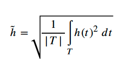
The normal average function is not all that useful of a measurement because any AC signal will average out to 0 over a cycle. The RMS is a much more useful measurement because it is positive definite and a voltage signal h(t) will deliver the exact same power to a resistive load over a time interval T as a DC signal at a level of h̃. Suppose that h(t) can be expressed as sum of sine waves with various amplitudes, frequencies, and phase shifts, so that:

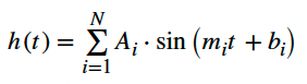
This means that

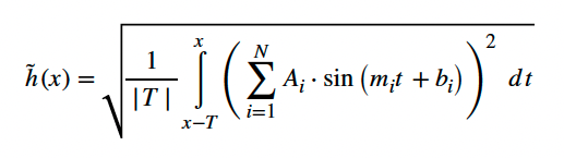
We can clean this up a little bit by scaling everything so that T = 1 cycle of the fundamental 60 Hz line and rearranging the terms to get:

The key to understanding what happens to the rms reading under various conditions is the innermost integral expression, which is the integral of the product of two arbitrary sine waves over a single cycle:

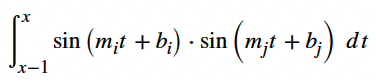
It is helpful to define a new function f(x, m, b) in terms of time variable x, frequency variable m and phase shift variable b that will figure prominently in the evaluation of the integral. Let:

Another notation that will become useful is to write subscripts of sum, diff, and prod on variables to correspond to the sum, difference, and product of the corresponding i and j variables, so m_sum = m_i + m_j, m_diff = m_i – m_j and m_prod = m_i · m_j. Then, skipping a lot of algebra steps, the expression is equivalent to:

This formula is the main result and all the odd behavior in rms readings from interharmonics can be seen in this formula. Here are several important takeaways.

As the frequency m approaches 0, in equation 4, the expression for f approaches $\frac{\cos(b)}{2}$ .

The expression for f is just a pure sine wave with frequency m. Both the amplitude and the phase shift now depend on the input frequency, but there’s no change in shape or any weird distortion effects.

When the frequency is some harmonic multiple of 60 Hz, the expression $\sin\left(\frac{m}{2}\right)$ in the definition of f is exactly 0, so f = 0.

When the two input waves have different frequencies, then the result of this integral is one sine wave with a frequency of the difference of the two input frequencies and one sine wave with a frequency of the sum of the two input frequencies. As an example, suppose there is some 25 Hz signal and some 40 Hz signal on the line. Then, this integral will produce some 15 Hz effect and some 65 Hz effect.

When the two input waves have the same frequency m, then the result is $\frac{\cos(b_{\text{diff}})}{2} – f(x, 2m, b_{\text{sum}})$ which has a DC offset and a 2m sinusoidal component.

When the two input waves have the same frequency m and same phase shift b, then b_diff = 0 and the result is $\frac{1}{2} – f(x, 2m, 2b)$

When the two input waves have the same frequency m, the same phase shift b, and the frequency is an integer multiple of half the line frequency or 30 Hz, then the f(x, 2m, 2b) term drops out and we are left with just $\frac{1}{2}$.

When the two input waves are both harmonics of the 60 Hz line, then both m_diff and m_sum are also 60 Hz harmonics and the whole expression becomes 0.

Notice that the dependence on x drops out in the previous two notes, meaning that the 60 Hz line and all of its harmonics only ever contribute DC components to the RMS calculation. Sampling at any point in the 60 Hz cycle and computing rms over the last cycle is exactly the same as starting at any other point in the cycle.

Conversely, interharmonic signals present with the 60 Hz line will cause variation in RMS measurement from cycle to cycle as well as within a cycle.

We can complete the calculation for rms by substituting the result of the integral into the equation and we see that given an input h(t) which can be represented by a sum of sine waves, the rms at a point x over the last cycle is given by:

Worked Example

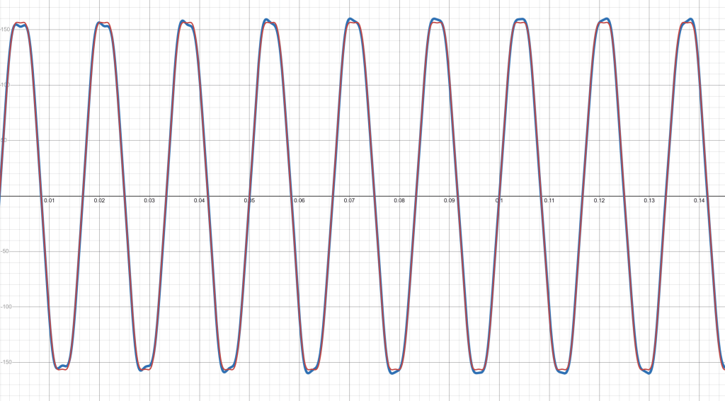
Suppose at some 120 V_rms service, there is a 5% 3rd harmonic signal and an inverted 3% 5th harmonic signal, which is not uncommon especially in AC to DC conversion and it causes the peaks of the waveform to flatten out a little bit. On this service connection, there is also some weird machine that injects a 2% signal at 175 Hz. Figure 1 shows a graph of this function, where the blue waveform shows 175 Hz distortion and red does not show the 175 Hz. This example will work out the RMS of this curve at a point x over the last 60 Hz cycle from x.

First write out the signal h(t) where t is in units of seconds:

Now, I will substitute this into Equation 6 and divide both sides by two factors of 120 to get

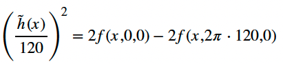
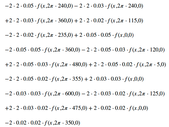
Now substituting all the f(x,0,0) terms with $\frac{1}{2}$ and all the harmonics of 50 Hz to 0, we get

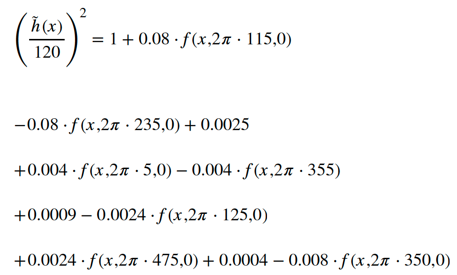
Figure 2 shows a plot of this example. Notice that there is a strong 5 Hz component of the signal and that it quickly oscillates between two 5 Hz sine wave boundaries. This will very likely cause a serious problem with flicker. There is a maximum of a 0.44% voltage drop on a 5 Hz basis.

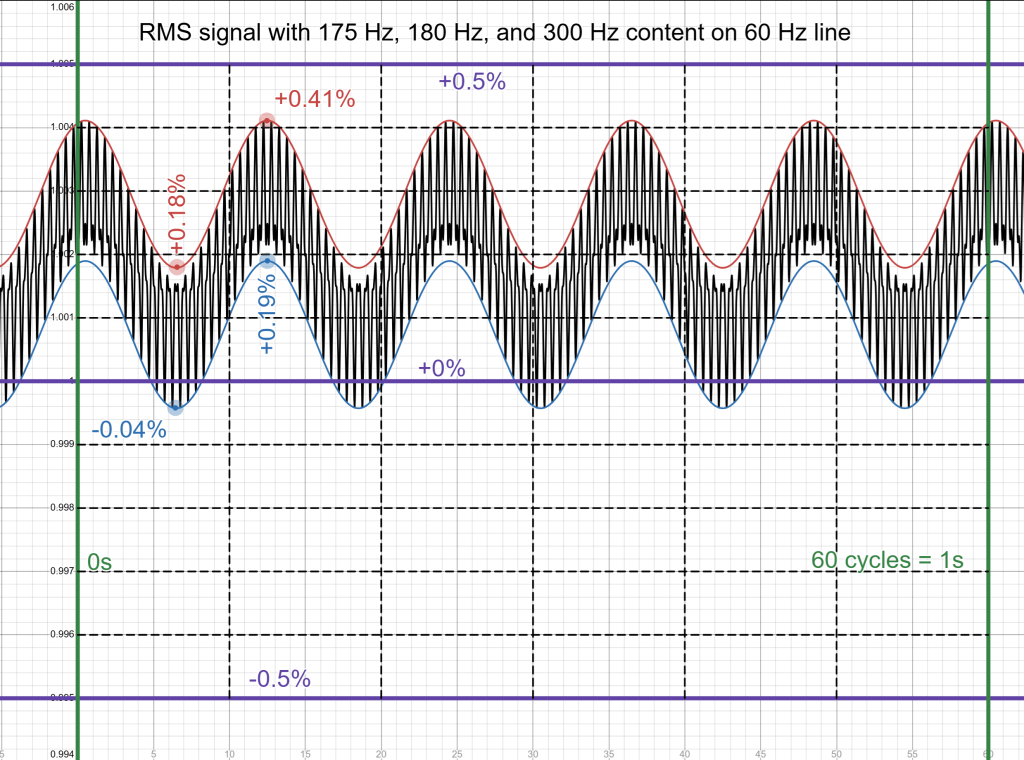
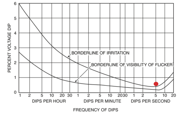
Figure 3 shows the IEEE 141 standard of Visibility and Irritability for flicker. I have placed a red dot on the graph roughly where this example would be measured, which is inside the region of irritability. Humans are incredibly susceptible to 5 Hz variations in light intensity and it does not take very much variation to become intolerable. All of this oscillatory strangeness would disappear altogether if the 175 Hz injected signal were to be removed and the RMS graph would just become a horizontal line.

Conclusion

If a signal is decomposed into a sum of sine waves, then the RMS calculation involves a bunch of integrals of a product of two sine waves. This integral yields two waves, one with the frequency of the difference of the two inputs and one with a frequency of the sum of the two. With just a 60 Hz line and integer harmonics of the 60 Hz line, most everything cancels out nicely and the result is just a DC value. Interharmonics are different and this nice cancellation does not apply. One major effect of this time varying aspect of the RMS calculation with interharmonic signals is light flicker.