Ferroresonance and Power Quality

Abstract

Most in the world of power quality are familiar with the concept of resonance in an electrical network as well as the methods for dealing with the issues and byproducts of resonances. Ferroresonance, on the other hand, is less well-known, the results of which can lead to significant issues including distribution equipment failure.

This whitepaper aims to give a high-level overview of ferroresonance, and how to potentially identify this anomaly when it presents itself in a power quality recording.

Overview

Linear resonance is an electrical phenomenon that occurs at the frequency where the inductive and capacitive reactances are equal in magnitude. See equation 1. This is a phenomenon of linear circuits:

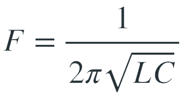
Ferroresonance, however, has a more complex set of dependencies. As the name implies, ferroresonance has as a significant factor the initial magnetic flux of a transformer’s iron (ferro-) core. Note, too, that ferroresonance is being contrasted with linear resonance, indicating that ferroresonance exhibits nonlinear behavior. In some instances, non-linear behavior can be modeled with linear approximations. This is not the case with ferroresonance.

In general, ferroresonance happens when circuit capacitance from shunt capacitor banks, series line compensation capacitors, cable capacitance (especially from underground runs), or other sources, interacts with a transformer inductance. The nonlinear aspect arises due to the nonlinearities in a transformer core. A transformer under light load conditions exhibits a nonlinear inductance, where the core losses and magnetization current are a significant fraction of the total load. A transient or other normally minor disturbance can excite the resonance formed by the system capacitance and instantaneous transformer inductance. The effects of the resonance itself can change the instantaneous transformer inductance, providing a mechanism for nonlinear feedback and a sustained problem. The result can be severe voltage issues, including overvoltage (over 3 times nominal voltage) and very high voltage distortion, where the nonlinear “ringing” is closer to an oscillation at a non-powerline frequency.

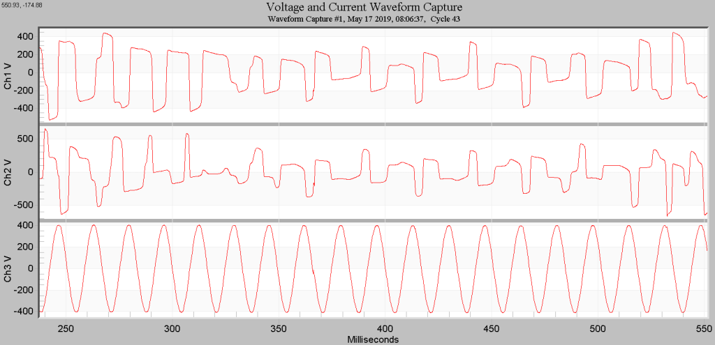
Figure 1. Ferroresonance on Phases A and B

If there is no (or a very small) resistive load connected to the network and one phase is interrupted, ferroresonance may ensue. It should be noted that if the remaining phases are not brought offline quickly thereafter, equipment failure may occur as a result of over-voltage.

A good rule of thumb for determining whether or not ferroresonance is possible is to look for: (1) the presence of a capacitance in series with the transformer’s magnetizing inductance (cap banks or capacitive coupling) and (2) an unloaded (or low load) transformer (<20% of the rated load).

Symptoms can run the gambit with ferroresonance, however in this particular instance (the recording that is analyzed in this white paper) the customer noted that breakers were continuously tripping.

Analysis

When ferroresonance is suspected a PQ recording should be undertaken. The recording should be configured to record, at a very minimum, triggered waveform capture (>= 5% THD will be sufficient, as instances of ferroresonance will yield THD in the hundreds of percent), 1 second RMS stripcharts, voltage THD stripcharts and phase angle stripcharts.

An example from a commercial customer is presented in the following figures. This customer is served by a 1.5 MVA pad mount transformer. For this recording, the transformer was unloaded, and a single phase event was created to test for the possibility of ferroresonance. The primary was 34 kV, and the connection wye-wye. Ferroresonance was triggered on phases A and B, as can be seen in Figure 2. Phase C is normal, while phases A and B are closer to square waves, with wildly fluctuating levels. The data in this file has been exported for further analysis in Python below.

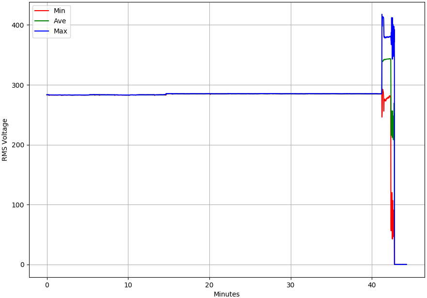
Figure 2. RMS Average Stripchart from Recording with Documented Instance of Ferroresonance

A quick glance at the RMS Voltage stripchart usually provides evidence of a problem. Figure 2 shows a stripchart trace pulled from a recording with a known instance of ferroresonance. Note that for the bulk of the recording (the first ~40 minutes) the RMS voltage is hovering around a nominal of 280V. Things take a drastic turn for the worse approximately 15 minutes from the end of the recording.

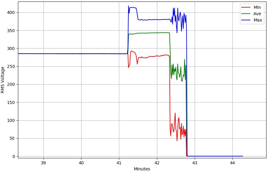
Figure 3. Wild Voltage Fluctuations Reflected in the Steady-State Voltage in RMS Voltage Stripchart

Note in Figure 3 the wide disparity between minimum and maximum RMS values in the graph. These large swings (in this instance ~350V over the course of three minutes) are good first indicators.

After taking a look at the stripchart records and noting these wild voltage swings, the next logical step is to look at the waveform capture records. Waveform captures are an indispensable part of ferroresonance analysis. (Both the Revolution and Guardian product lines at PMI provide high frequency sampling for resolution up to the 127th harmonic (7.6 kHz) for detailed waveform analysis.)

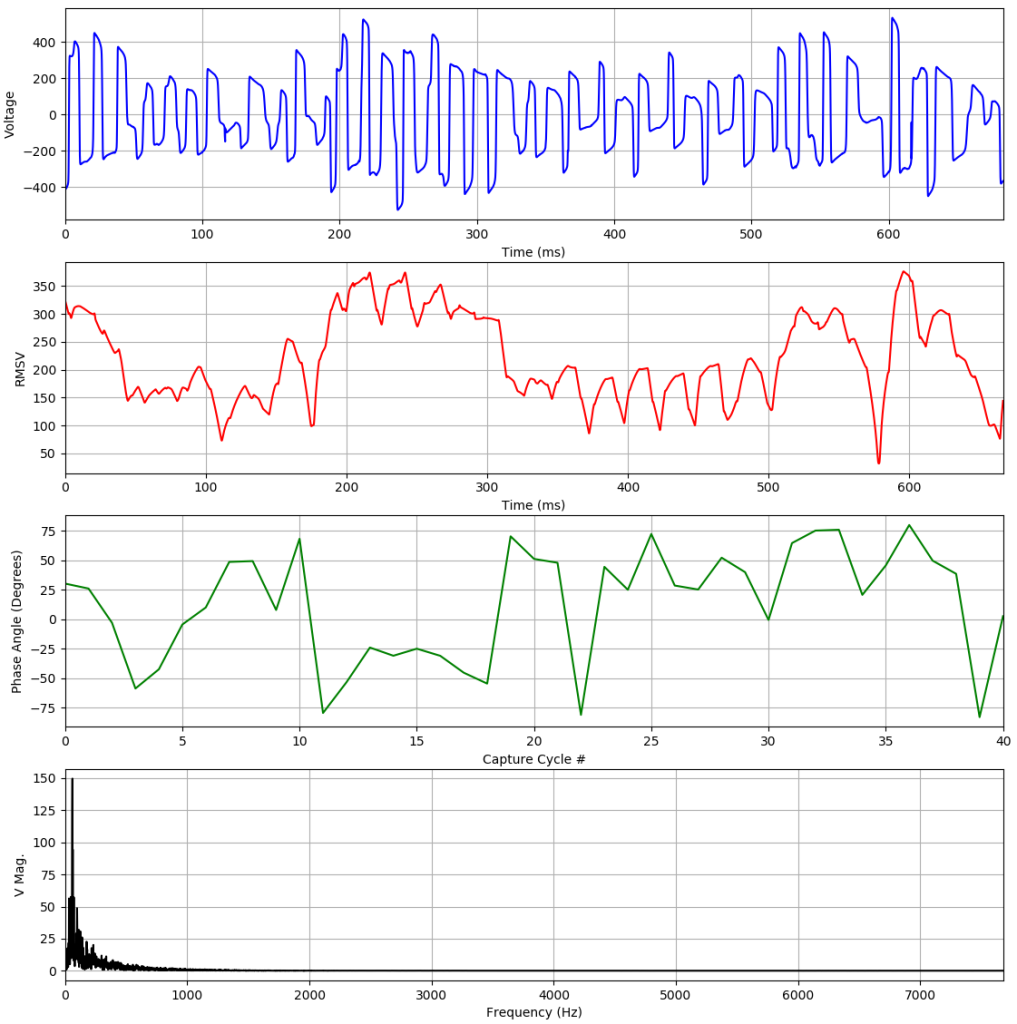
Figure 4. Snapshot of a Waveform Capture from a Confirmed Instance of Ferroresonance

The first plot in Figure 4 is the instantaneous voltage in the time domain. The second plot is a running series of point-by-point RMS for the sample width through all cycles. The third plot is a cycle-by-cycle comparison of phase angle. There were 41 cycles recorded in this particular waveform capture. The final plot contains the frequency analysis from the FFT of the full 41-cycle capture.

A quick glance at Figure 4 shows some startling graphs. (Note the description in the figure for a plot-by-plot breakdown of what’s being displayed in each plot.) All four plots should really stand out as anomalous. The “boxy” shape with nearly flat waveform crests is a great visual indicator of ferroresonance. When looking at the FFT results (plot 4) the reader will note that there’s a high DC component present in the frequency domain – this will help account for the flattening seen in the time-domain.

Note also that there are significant magnitudes for all frequencies up to about the 13th harmonic (780Hz). This will yield THD values of over 100%.

The second plot in the graph is a return to the RMS Voltage stripchart that was studied earlier. The recording interval from the strip chart was 1 second, so what’s being viewed in this plot is a little more detailed. (It’s a sliding window of sampling width through the full 41 cycles in the waveform capture. The full duration right at about 700ms, so the full graph in this plot is less than the “width” of a single point from the RMS V stripchart graph from above.) Wild voltage fluctuations can be seen here and in much greater detail. Again, this is a 280V nominal and the RMS Voltage varies from a minimum of about 48VRMS to a maximum of about 365VRMS. While the under-voltages are worrying, the over-voltages are far more significant (equipment failure, cable insulation failure, etc.).

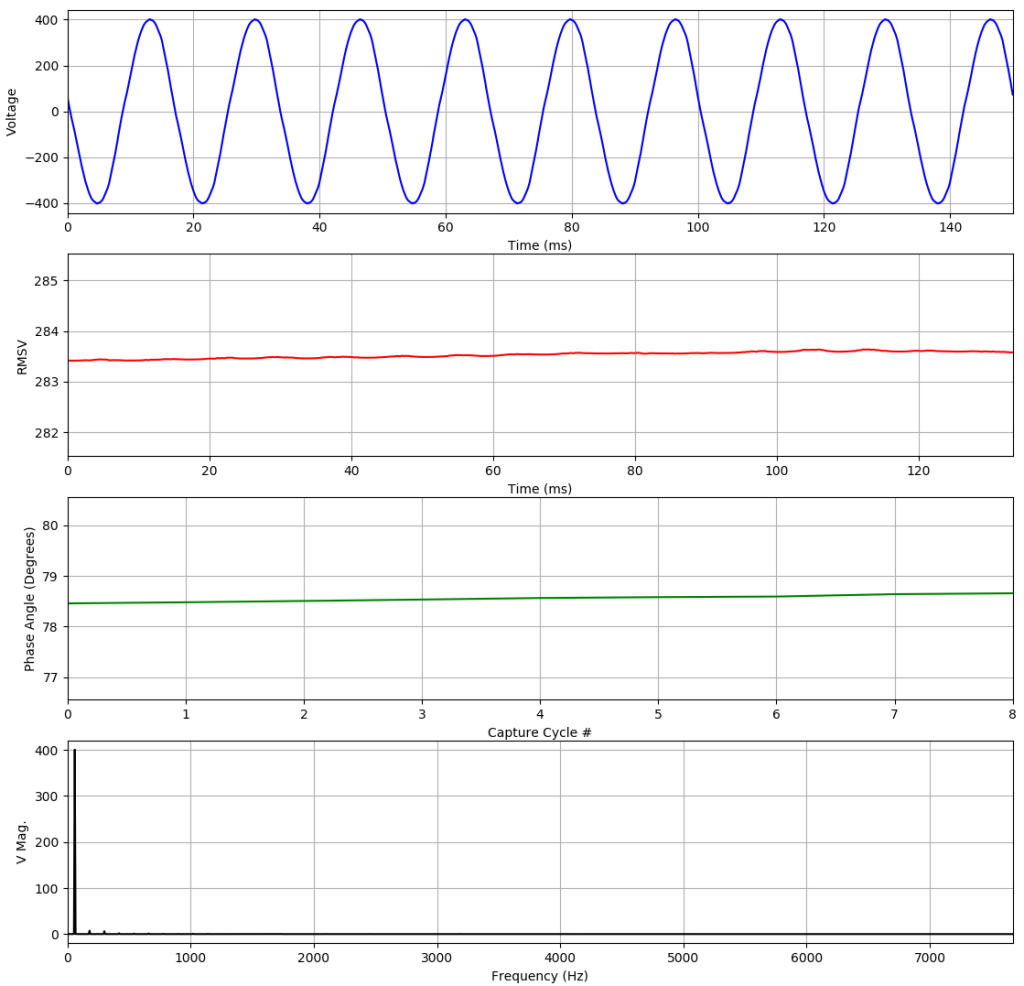
For comparison, a “sane” capture from the field is provided in Figure 5. Take special note of the steady RMS Voltage and phase angles (and lack of significant harmonic distortion in the frequency domain).

Figure 5. A ‘sane’ Capture from the Field Showing a Clean Capture for Comparison

Prevention

Ensuring that a transformer is at least 20% loaded (ideally with resistive loads) can help avoid ferroresonance. This is especially important during transformer energization. Loss of a phase, or single pole switching (which could briefly energize only one or two inputs) can also trigger a ferroresonant condition. Avoiding single pole switches, and favoring 3 phase breakers vs. single phase fuses can help prevent this.

NOTE: Devices that are not active in the system are disabled. Disabled devices cannot be selected for “bursting”, even using the “Select All” checkbox feature. Disabled devices will appear grayed out in the Device List.

Conclusion

Ferroresonance is a somewhat unusual phenomenon resulting from the interaction of circuit capacitance with the nonlinearities of a transformer’s “inductance”. While instances are uncommon, engineers should be aware of the symptoms, causes and effects of these types of events. This white paper has provided some recommendations for capturing instances of ferroresonance with power quality recorders and has provided some good first steps in analytically identifying instances of these potentially hard-to-diagnose events.

Notes

The graphics in this image were the product of a Python library that PMI supplies free-of-charge (upon request) from power users who wish to dive a little deeper into PMI’s power quality recording files. Fully commented and documented copies of the scripts and libraries used to generate these images can be obtained by contacting PMI Technical Support at support@powermonitors.com and requesting our PMI Python analysis library. For a detailed description of what’s available in these libraries, see the following whitepapers: Advanced Waveform Analysis Using Python and Analyzing Power Quality Data with Python.