Abstract

The first step in voltage sag mitigation is finding the source of the sag. In a power quality recording, spotting the voltage sag itself is often easy, but determining whether the sag was caused by a load being monitored (downstream), or incoming from the distribution side (upstream) requires a closer look at the data. Techniques for determining the sag location are described in this whitepaper, along with examples.

Voltage Sag Basics

A voltage sag is defined by IEEE 1159 as a “decrease in RMS voltage to between 0.1 and 0.9 pu at the power frequency for durations of 0.5 cycle to 1 minute.” Voltage sags are a result of Ohms law: V = I x R. Current flow caused by brief, excessive current from a load, or system faults creates a voltage drop across all impedances in the system (wire resistance, transformer impedance, connections, etc.) Referring to Figure 1, the “Source Voltage” Vs is the theoretical zero-impedance AC supply, which can be approximated by the substation transformer for many customer-induced voltage sags. For fault currents or origination upstream from the substation, the transmission system may be considered the voltage source. R represents the total resistance through the distribution system to a customer load, depicted as a motor in Figure 1. The current drawn by the load is I, which flows in a loop from Vs, through R, the motor, and back to Vs. Ohm’s law gives voltage drop V across the total resistance R. The voltage applied to the load is the sag voltage, Vs – V. Any voltage drop in the system subtracts from the nominal line voltage, reducing the voltage delivered to the load.

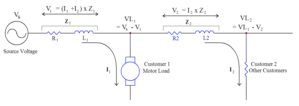
In the simple case of Figure 1, the load itself is also the cause of the sag. A more complex, but typical case is shown in Figure 2. Here two customers are involved, drawing currents I1 and I2. The current sourced by Vs is I1+I2. The total current produces voltage drop V1 across the impedance in common to both loads. Current I2 products further drop across the line that separates the two loads. Customer 2 sees the largest drop, but customer 1 also sees a drop due to customer 2, but only from impedance Z1.

Because all equipment downstream of the sag source are electrically in parallel, the sag will affect all loads downstream from that point. A real scenario is often more complex, where customers also have their own wiring resistance producing voltage drops that are not shared by other customers.

If Customer 2 is experiencing problems due to voltage sags, a natural PQ monitoring point is at Customer 2’s service entrance. Recorded voltage at that point will reveal the frequency and depth of any sags. Just as importantly, monitoring the load current will reveal clues about whether the sag is caused by a load at Customer 2, or upstream (e.g. possibly at Customer 1).

Sag Voltage and Load Currents

The key in determining the sag source direction is the relationship between voltage and current during the sag. Here “upstream” is defined as closer to the voltage source electrically, and “downstream” defined as towards the end of the distribution line, but such that the PQ monitor’s CTs include the load current. For example, with a monitor at the base of a distribution transformer, upstream would be the anywhere on the primary side, and any customer load on the secondary would be downstream. The upstream/downstream question often reduces to “incoming from distribution” or “induced by customer load”, with the demarcation point being the secondary, service entrance, or point of common coupling.

Generally, there are four types of patterns seen:

1. Resistive loads, where the current drops during the sag
2. Constant power loads, where the current is unchanged, or rises slightly during the sag
3. Loads that switch off during the sag, where the current drops to zero
4. Loads causing the sag, where the current spikes to high levels during the sag

In the first three cases, the loads are reacting to the sag. In the latter case, the load is the cause of the sag. Importantly, in the latter case the load causing the sag must be downstream of the PQ monitor, since the current is present in the recording. In the first three cases, the offending sag current isn’t present in the recording. Since it must be present somewhere (otherwise there would be no sag), it must be upstream from the monitor.

For a constant resistive load, the load current during the sag is very simple, and follow Ohms law: as the voltage drops, so does the current. Incandescent lighting, resistive heating elements, and other linear loads will consume less current with less applied voltage. The nominal current returns as soon as the voltage returns to nominal. In a graph the RMS current will drop during the sag with no increase, immediately ruling these loads out as a sag source.

For a constant-power load, such as an electronic switch-mode power supply (SMPS), AC motor, or variable frequency drive (VFD), the current will (roughly) increase during the voltage drop. This increase is often fairly small, and the extra voltage drop from it is small compared to the sag depth itself. A SMPS or VFD will increase the pulse modulation frequency or duty cycle to deliver the same power with a reduced DC bus voltage present during the sag, thus increasing the load current. A directly-connected AC motor will also show an increase in current, although the effect is more dependent on the sag depth, motor speed, and motor load.

Some loads will disconnect during a sag. Motor contactors may drop out if the sag last more than a cycle, and intelligent controllers often intentionally disconnect a motor if the incoming voltage is outside the operating window. This will appear as an abrupt drop in current, and is often the source of the customer complaint.

Finally, a load that’s causing the sag will show a large current increase during the sag. The voltage drop must come from a large current source, given the low system impedance, and this surge in current should correlate exactly with the voltage sag. This is the pattern to watch for in the RMS stripchart graph.

The monitored current is usually a mix of all these load types, especially for different sag sources. The one constant is that if the sag source is downstream of the recorder, the current spike producing the sag will be in the recording, since all downstream loads are in parallel, and in series with the PQ monitor, by definition. There will be a large current spike at the same time as the voltage sag, as per the fourth case above. If the sag source is upstream, the voltage sag will be present, but the monitored current will only show other loads reacting to the sag, not the excessive spike causing the sag. These load reactions may be slight increases or decreases in current. The sag depth is related to the system impedance, which is roughly constant at 60 Hz, so a comparison of a suspected sag-inducing load’s current with other similar current spikes and corresponding voltage changes can help reveal if an increase in current was the cause or effect of a sag.

Examples

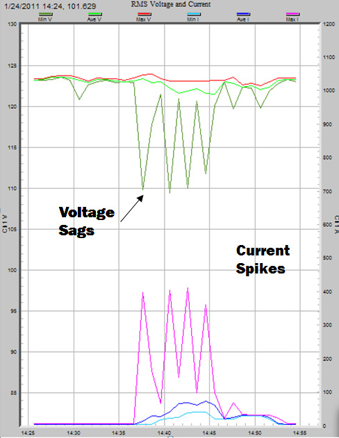
A clear example is shown in Figure 3. Here a single channel of RMS voltage is graphed with RMS current. The one cycle min and max, along with average values are displayed; the top three traces are voltage, the bottom three current. Four voltage sags, indicated by the dark green dips, occur at the same time as four current spikes (purple). The magnitude of the sag is directly related to the magnitude of the current and depends on the system and load impedance. In this example, a 400A current spike produces a 14V drop (to 0.88 pu), giving a 14V/400A = 0.035 ohm resistance.

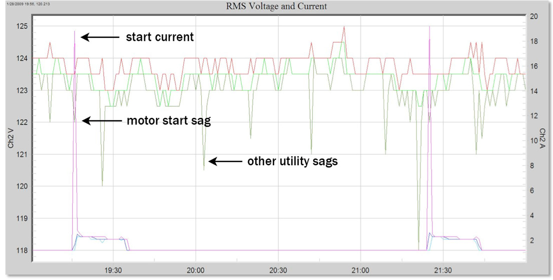
A more complex case is shown in Figure 4. A small motor produces a 19A starting current which results in a 1.5V sag during the motor start. Deeper sags are also present, with little or no corresponding change in current. The load producing those sags is upstream from this PQ monitor.

One pattern to watch out for is an apparent voltage/current correlation that is not always present. Unless the system impedance changes, a specific current spike amplitude should produce roughly the same voltage sag every time. If that’s not the case, then the current being monitoring is likely not the sag despite an apparent correlation. In Figure 5, the large 20V sag is perfectly lined up with a 42A current spike. However, other nearby current spikes to similar levels only produce 1V sags. Unless the system impedance changed by a factor of 20X during that large sag, the load current is not the source. More likely, the load responded to the sag, e.g. a motor restarting due to a contactor dropping out. It’s also possible that a loose/intermittent connection really did cause an increase in the system impedance during that time, but a motor restart is more likely in this case.

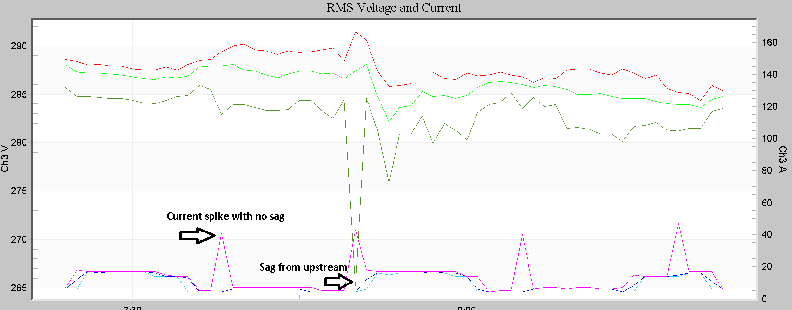
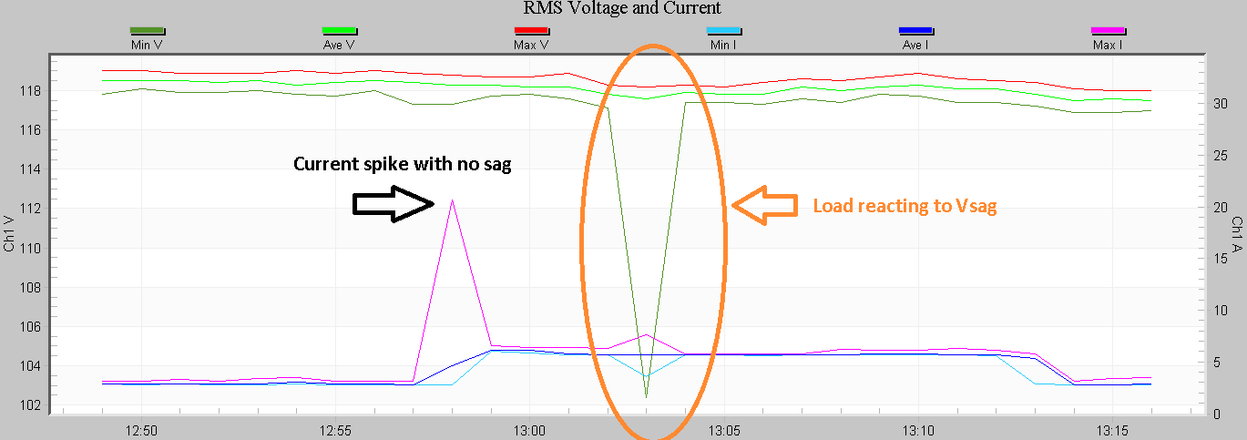
Another example is seen in Figure 6. Here a current spike to 20A produces no visible voltage sag. A few minutes later, a deep voltage sag (0.85 pu) occurs while the current min value drops and the current max value increases slightly (2A). This small spike could not have caused this voltage drop, if the much larger current spike didn’t produce an even deeper sag. These loads were responding to the voltage sag, not causing it.

Conclusion

The key to locating voltage sag sources in PQ data is the relationship between sag voltage and current. A high current, either from a system fault or excessive momentary load current (e.g. motor start) is the root cause of a voltage sag. If the offending source causing the sag is downstream of the monitor, its high current will be included in the data along with all other downstream loads. Its current will appear as a spike in an RMS stripchart, exactly coincident in time with the voltage sag. If the source is upstream, the voltage sag will be present, but the monitored current will only show other loads reacting to the sag, not the excessive spike causing the sag. These load reactions may be slight increases or decreases in current. The sag depth is related to the system impedance, which is roughly constant at 60 Hz, so a comparison of a suspected sag-inducing load’s current with other similar current spikes and corresponding voltage changes can help reveal if an increase in current was the cause or effect of a sag.