Voltage Sags in Photovoltaic Systems

Abstract

Photovoltaic (PV) generation is electrically in parallel with the utility supply, and thus lowers the steady-state system impedance. The ideal result is a reduction in locally caused voltage sags as the PV system supplies power to high-current loads. The actual result can be an increase in voltage sag severity, due to the design of typical PV inverters. The reasons for this unfortunate result are presented here, along with a real-world example.

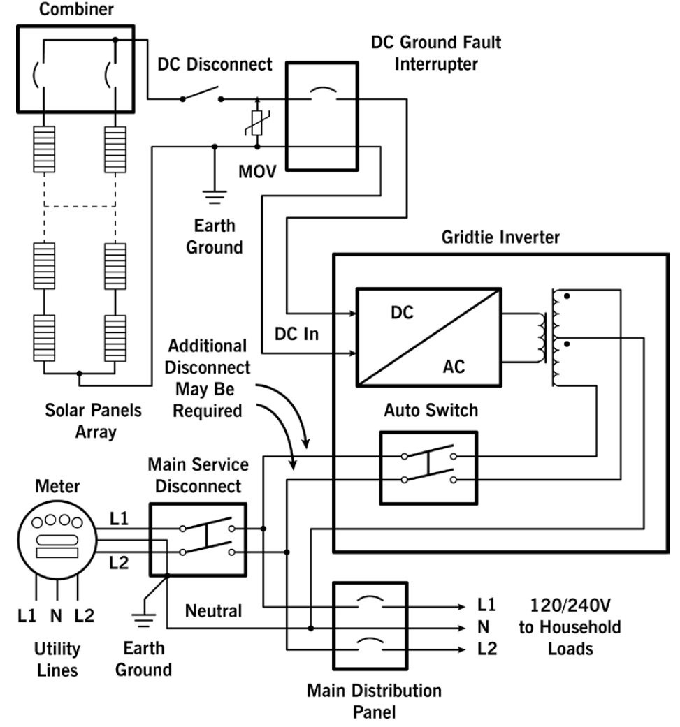
A PV system consists of several components, including the panels themselves, interlocks and switches, and in particular, a DC->AC inverter (see Figure 1). The raw PV output is DC; the inverter converts this to a 60 Hz sinusoidal voltage waveform. Because the inverter output is connected in parallel to the distribution transformer secondary, the amplitude and phase of the inverter output must be carefully controlled and adjusted to match the utility voltage. The inverter must target an amplitude slightly higher than the utility voltage to supply positive power to any attached loads (or loads upstream). Generally, the output phase angle is targeted to match the utility voltage so that the inverter only supplies real power (rather than reactive power).

Figure 1. Typical PV system, with inverter, disconnect, and panels

Simple Distributed Generation Model

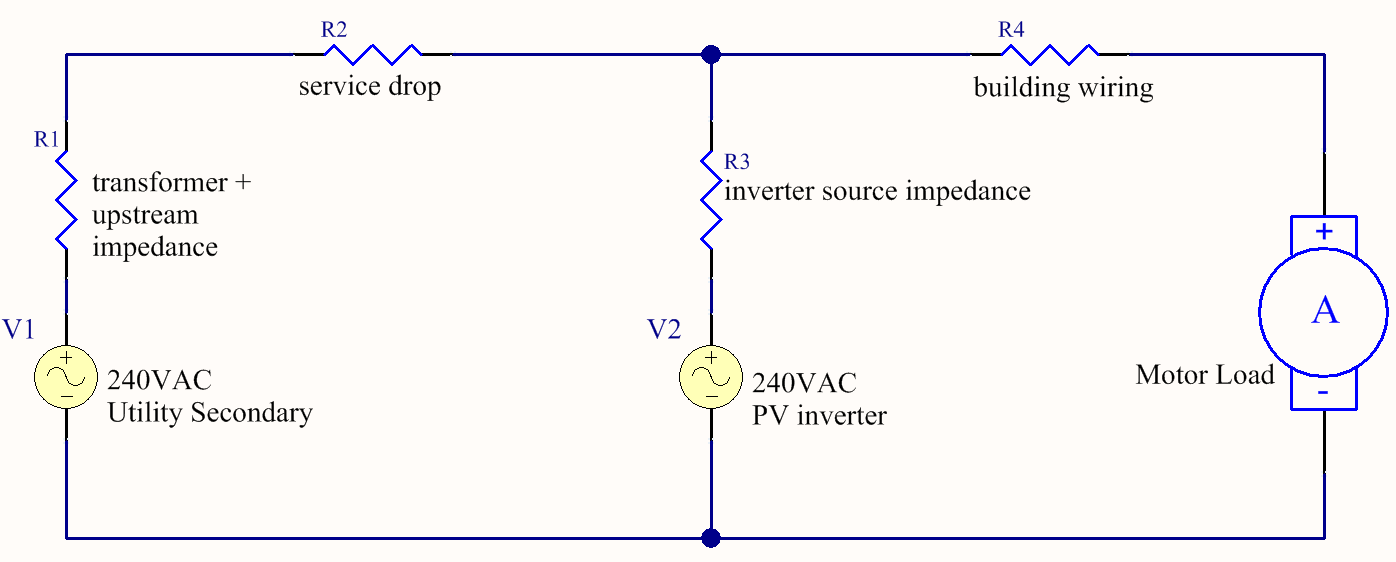
A simple analysis of adding PV generation in parallel with the utility source is shown in Figure 2. Voltage source V1 represents the incoming utility voltage from the transformer secondary, with associated source impedance R1. R2 and R4 model the wiring and connection resistance for the service drop and internal wiring to a high current load, shown as a motor. The PV system is modeled as an ideal voltage source V2, with output impedance R3. A rough estimate of R3 for a 5 kW system would be 240V / (5000/240) x 0.05 (5 per unit) = 0.6 ohms. That gives a 5% voltage drop at full load (20.8A). This is considerably higher than R1, which could be around 0.03 ohms for a 25 kVA transformer.

Despite the fact that the utility voltage is much stiffer (i.e., lower source impedance) than the PV system, adding any voltage source in parallel should only help with voltage sags. Roughly, a 5 kW PV system could be expected to reduce voltage sags by around 5% when placed in parallel with a 25 kVA transformer secondary. A long service drop would make the PV system even more effective inside the building.

Figure 2. Simple utility + PV generation model, assuming ideal sources and linear source resistances

This simple model of an ideal voltage source and linear resistance is a good first-order approximation for incoming utility power. The upstream generation capacity is very large compared to any local load, and series resistance is accumulated from actual wire and connection resistances with a high short circuit current capacity. Applying a very low load resistance momentary (e.g. a motor start load) will result in a very high current, and increasing voltage drop, as predicted by the simple model. At the extreme, a dead short will produce very high short circuit current (until an upstream fuse or breaker interrupts the line).

PV Inverter

Unfortunately, a real-world DC->AC inverter is not well modeled by an ideal voltage source with linear source resistance. The synthesized AC waveform is created by switching transistors, much like a variable frequency drive (here producing AC instead of DC or motor pulses). The switching architecture is a very nonlinear system, with output impedance roughly correlated to the switching frequency while the output current is within the design parameters of the inverter. The sun loading on the panels also affects the effective source resistance. Inverters have a peak current output which is related to the transistor and other circuit element limits and is often a hard limit imposed by the controller in real time. The peak current limit translates into a maximum crest factor, similar to a UPS. The inverter is not able to produce current much beyond that maximum.

To make matters worse at high momentary currents, the inverter is usually microprocessor controlled, including feedback for adjusting amplitude and phase output. This feedback is optimized for stability during steady-state conditions. In particular, a phased lock loop (PLL) algorithm keeps the synthetic 60Hz frequency phase parameters locked to the power line. These algorithms are often designed with sub-second time constants but are usually not fast enough to respond to voltage sags (or current surges) lasting just a few cycles. By the time the controller could adjust the inverter to the sag, the sag is over.

PV inverters may even disconnect during a sag. IEEE 1547, IEEE Standard for Interconnecting Distributed Resources with Electric Power Systems, calls for the inverter to disconnect within 0.16 seconds for a deep sag (under 50%). Similarly, UL 1741, Standard for Inverters, Converters, Controllers and Interconnection System Equipment for Use With Distributed Energy Resources, requires inverters to disconnect based on undervoltage conditions to prevent islanding. Voltage sag ride-through is a desirable feature for a PV inverter, but not always present or simple to implement. Ride-through is designed more to keep the inverter online at all rather than to actually help mitigate the sag. Here the best-case scenario is to avoid a complete loss of PV output during the sag, right when the circuit needs it most.

Real-World Example

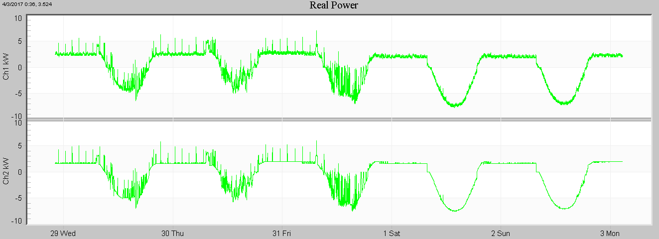
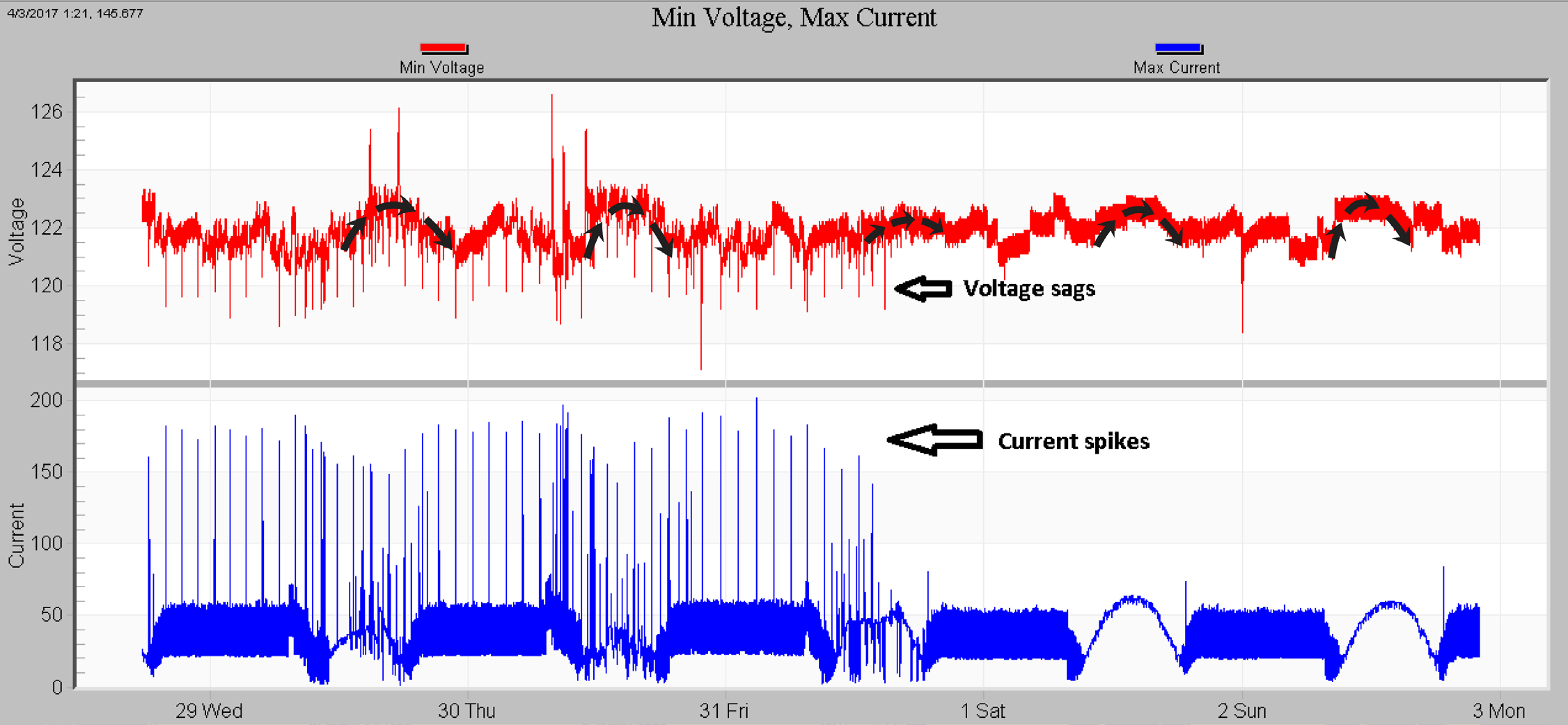
A real-world inverter output is shown in Figure 3. This is a single-phase commercial service with a 15 kW solar array. The two 120V inverter outputs are shown over a four day period, including a weekend. Power spikes are visible during the week, both night and day, and virtually none during the weekend (when there is very little activity at this location). An RMS voltage and current graph is shown in Figure 4. The top trace (red) is RMS voltage, showing one cycle minimum values at each stripchart interval. The bottom trace (blue) shows the one-cycle RMS current minimum. The overall voltage rises throughout the day as PV output increases (shown with thick dashed black arrow); the increase varies depending on the cloud level that day. A large motor on this secondary draws over 150A of starting current, creating a 2-3V voltage sag each time. These current spikes and voltage sags happen regularly throughout the day and night during the week, as indicated in Figure 4. Sags during the day are affected by the PV system. At night, the PV system is effectively out of the picture.

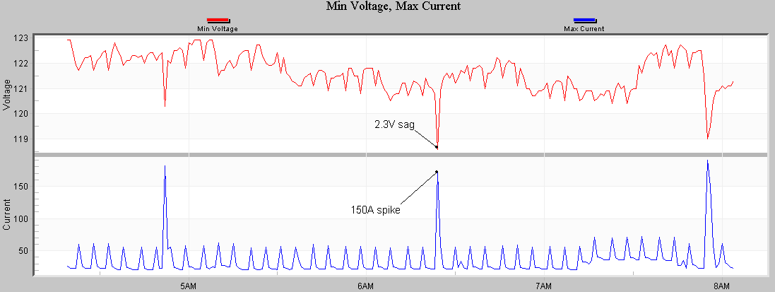
Figure 3. 10 kW single-phase PV output over 5 days

Figure 4. RMS voltage single cycle mins (red, top plot) with RMS current maxes (blue, bottom plot). 150A motor starts are causing 2-3V sags.

A typical night time sag is shown in Figure 5. Here the 150A motor starting current causes a 2.3V sag. Smaller sags can also be seen, with correspondingly smaller spikes in current. The PV system is not altering the circuit at this time of day (6:30am), so the sag depth is determined by the distribution transformer, service drop resistance, etc. A 2.3V change from 150A of current gives about 0.015 ohms as the source impedance, suggesting a 50 kVA transformer.

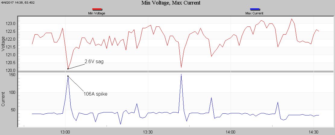
Figure 5. 2.3V sag from 150A current spike while PV system is idle

The same motor during the day is shown in Figure 6. The motor starting current seen at the monitoring point is the net current after the PV system has absorbed some of the load current. The net motor start current seen by the Revolution PQ monitor is 106A, with a 2.6V sag. A similar sag appears a few minutes later. These sags are at 1pm, near the peak PV output. Even though the PV system has “swallowed” 44A of the starting current, the voltage sag depth is actually worse than before. The effective resistance here is 0.025 ohms, 66% higher than before. Given the nonlinear nature of the inverter, it’s difficult to predict the effective impedance at other load currents or sun loads. The “resistance” is effectively a dynamic impedance that changes depending on load current, absolute voltage level, and sun loading.

Figure 6. 2.6V sag from 106A current spike while PV system is active

Conclusion

The sags shown here are only a few percent, with or without the PV effects. In a location with a larger PV system relative to the service size or deeper sags, the PV behavior becomes more important. At best the PV system will continue to ride through a voltage sag while absorbing current until the max crest factor or output current is reached. The voltage sag may be largely unchanged or could be even deeper than without the PV system. In the worst case, the PV system may trip offline during the sag, transferring any load it was absorbing back to the utility while the voltage is already low. Understanding that distributed generation is not as “sag friendly” as the utility system is key to dealing with PQ problems as these systems become even more widespread.

References

Inrush Transient Current Analysis and Suppression of Photovoltaic Grid-Connected Inverters During Voltage Sag, Proceedings of 2016 IEEE Applied Power Electronics Conference and Exposition (APEC)
High-Penetration PV Integration Handbook for Distribution Engineers, National Renewable Energy Laboratory (NREL)
Simulating the Dynamic Response of a Photovoltaic Generation System to Voltage Sags, CIRED 18th International Conference on Electricity Distribution