Abstract
The meteoric rise in the popularity of photovoltaic systems by both residential and industrial customers over the past several years has created a new series of power quality challenges for utilities. Among the ever-increasing list of questions being posed by utilities about the immediate effects of these photovoltaic systems is this: what are the effects of intermittent cloud cover as they relate to voltage regulation? The goal of this white paper is to answer that question by providing some concrete examples and graphs taken from measurements that have been collected over several months from diverse climatological regions in the US.
Voltage Distribution Without the Influence of PV Systems
Voltage delivered to customers is dependent upon two things: either the voltage as it is set from the substation or at a regulator mid-line and on the customers’ current loads. The effect of the customer current load influences the voltage on the distribution system wiring in an inversely proportional manner: as customer current load increases the voltage on the line decreases; as customer current load decreases the voltage on the line increases. This is due to V=IR losses in the distribution wiring, losses in transformers, etc. The customer voltage, VL, is the original system voltage VS, minus V1, the drop in the distribution system due to loading, as shown in Figure 1.

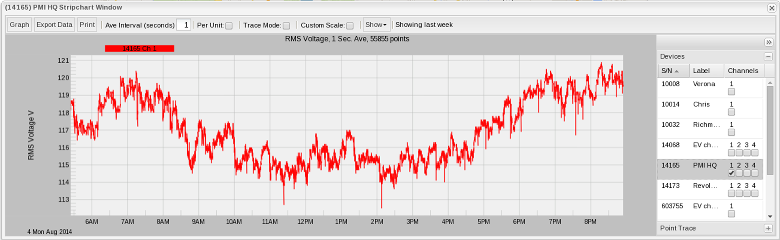
Figure 2 shows the voltage as measured from the panel at PMI. This graph shows the cyclical voltage fluctuations through the course of a week. What the reader will notice is that during the weekend (left-hand side of the graph) the voltage remains around the 120V nominal (+/- 2V in general). Then, as time progresses into the work week, the reader will see the following trend: in the early morning hours, the voltage remains around the 120V nominal – however, once employees start showing up at the facility around 0800 the voltage begins to sag. This is a result of the increase in PMI’s current load as facility lights, test equipment, soldering irons, computers, computer monitors and other equipment are powered on. At the peak of the work day voltage is hovering at around 114V. At the end of the day, after say 18:00, the voltage will return to close to the nominal as employees shut down their computers, shut off lights, irons, test equipment, etc. and return home.
Another interesting trend that can be noted in Figure 2 is that from 11:30 until 13:00 the voltage shows a slight increase – this can be attributed to users leaving their workstations and computer monitors going to “power savings mode” and office lights being shut off as employees head out to lunch, as shown in Figure 3.
Aggregate Load Prediction
Building on what was just discussed in the previous section, a utility can make generalizations about the aggregate demands of all customers on a distribution line for any given period of time. For instance, even though the graph in Figure 1 was just from a single phase inside of PMI, it is indicative of a standard load at a business. A residence would likely be almost the exact inverse: as spouses and children leave home in the mornings heading to work and school, lights get shut off, air conditioning units shut off (or at least do not cycle on as frequently), computers and televisions are turned off, etc. All of these things would be turned back on when they come home in the evenings after work and school.
With those assumptions in mind, it has traditionally been possible to predict the aggregate customer load. This is because the load varies slowly and smoothly even though individual loads (such as those at PMI) may be switched off and on abruptly. When taken in the aggregate, however, distributed over hundreds of customers (thousands of loads), the net result is typically a slowly varying, predictable load. Given this traditional load pattern, voltage regulation could be accomplished with simple timers on voltage regulators with peak demand being pretty well predictable.
Introduction of PV into the Equation
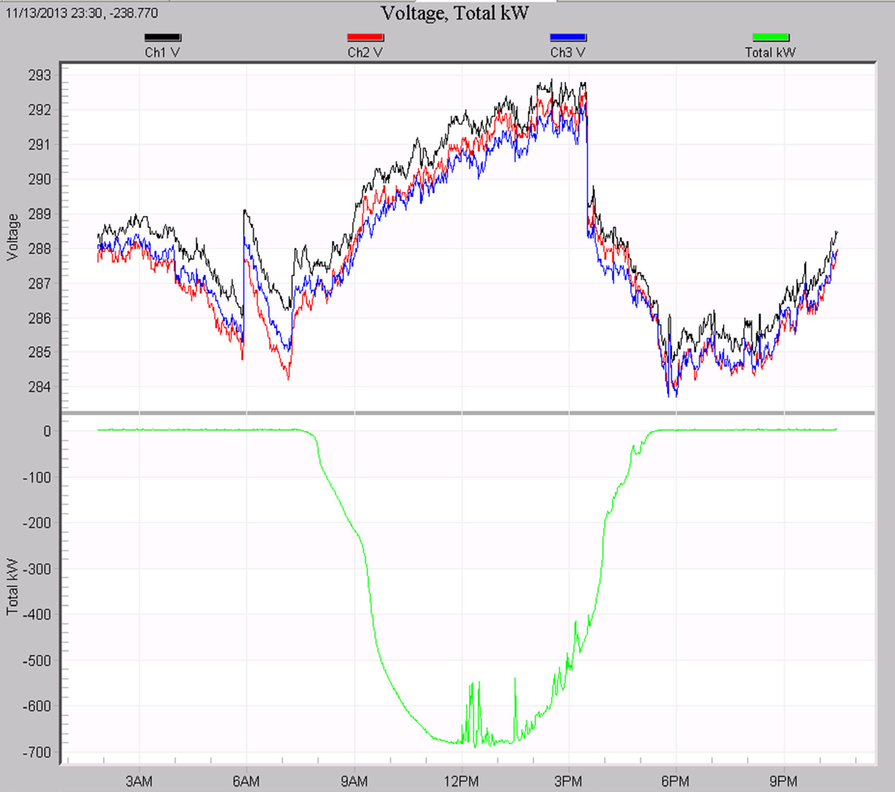
The base effect of extra PV generation can be seen in Figure 4, where the RMS voltage creeps up as the amount of generation increases. The voltage rises to 5% high, when a regulator makes a change to drop the voltage back to within limits. With unpredictable cloud cover, photovoltaic (PV) systems throw a monkey wrench into the traditional aggregate load prediction model. The new power now depends on customer load patterns (which typically hasn’t changed) and the power supplied by the PV system itself (referred to as “net metering”). The utility now sees the sum of the two. The local PV generation essentially “hides” the customer’s load while the sun is out (the customer’s load is being drawn from the PV system and not from the grid) and abruptly “reveals” the customer’s load when the sun goes behind the clouds (the customer’s load has now transitioned to the grid).
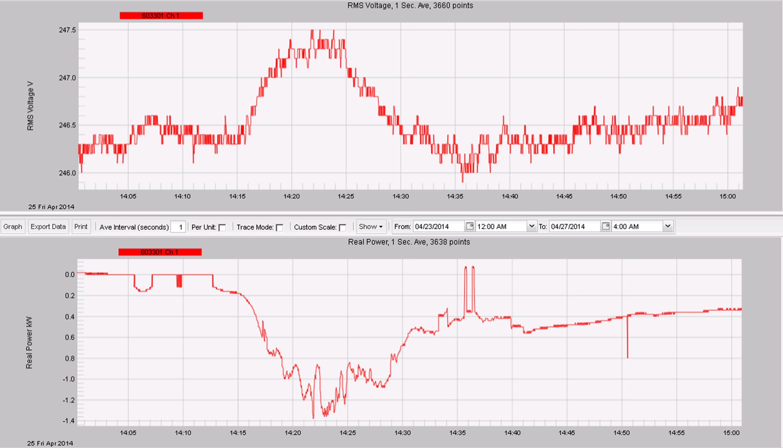
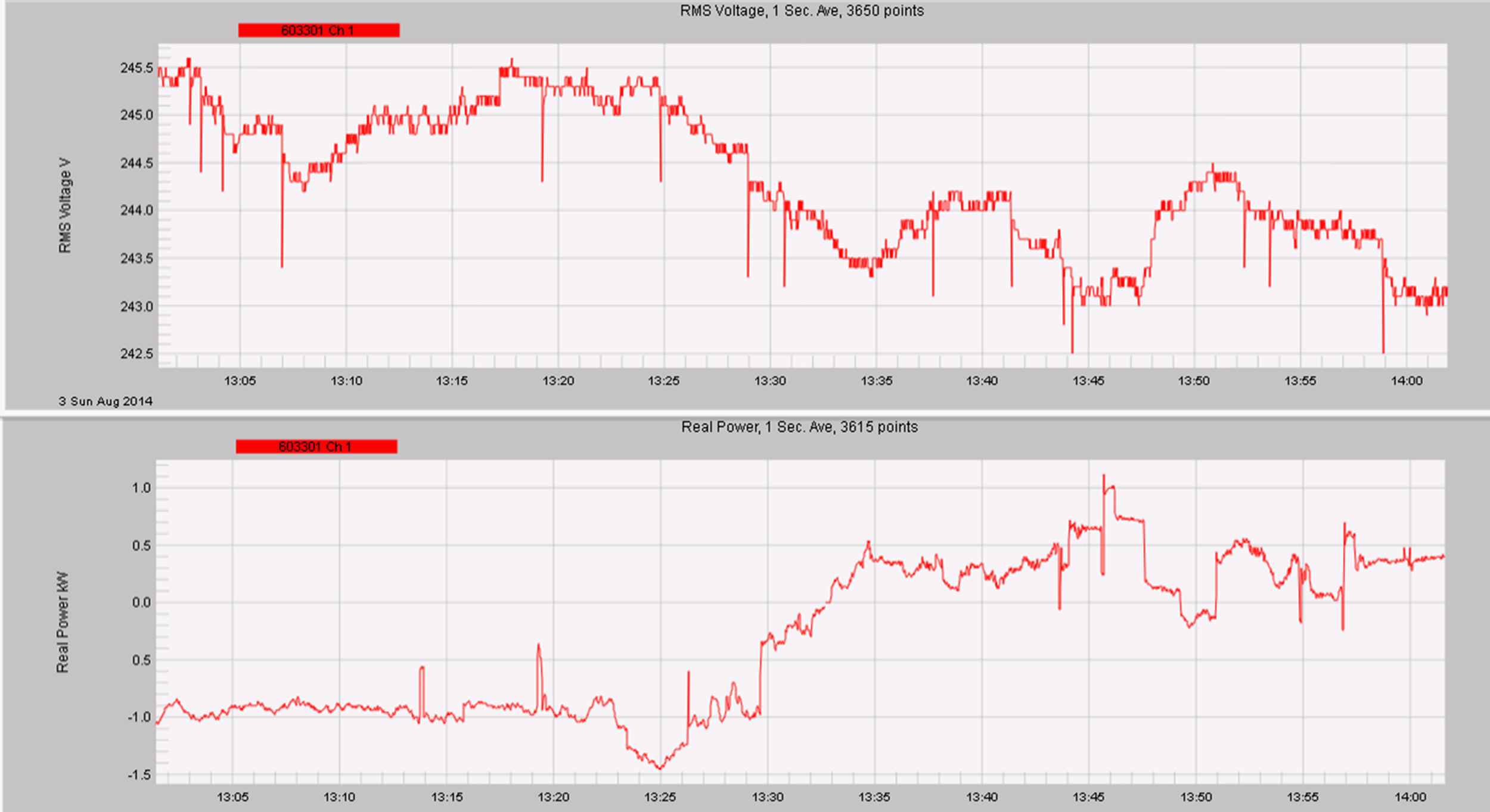
The problem here should be readily apparent: the traditional system of voltage regulation being easily predictable and adjustable at just a handful of times throughout a typical day has now gone out the window. Intermittent cloud coverage over PV systems can have very dramatic effects in PV output thus uncovering the true load (when the sun goes behind the clouds) or concealing it (when the sun comes back out) within the span of just a few minutes. In Figure 5, the sky is overcast in this residential neighborhood for most of the day, until around 14:00. The lower graph shows the net power from a single residential location, which starts to go negative around 14:10. The output peaks around 14:23, and then starts dropping as clouds obscure the sun. The RMS voltage is seen in the top plot. It rises about 1.5V for around 15 minutes while the sun is exposed, a change completely unexpected in a system without distributed generation. The opposite effect is shown in Figure 6. Here clouds reduced the PV output starting around 13:25, with a drastic change over the five minutes from 13:30-13:35. The RMS voltage (top plot) drops accordingly, due to the increased load in this area. The RMS voltage change is about 1.5V, out of 240V. As PV generation becomes a larger percentage of the total generation, this effect will become more prominent.
Net Results of Intermittent Cloud Coverage on PV Systems as It Relates to Voltage Regulation
The net result of these rapid fluctuations in production in PV systems is a demand for fairly quick adjustments from voltage regulators, cap banks, etc. to keep the steady-state voltage within limits. Most traditional equipment is not designed to make these rapid changes and would result in the utility needing to either upgrade to more robust equipment or add some near real-time sensing and control to handle the fluctuations.
An example would be to deploy dozens of sensors throughout the grid at “points of interest” (such as PV systems that had the potential to induce large swings in voltage on the distribution line) all of which would be feeding triggered readings (i.e. when a voltage, current or power reading is measured outside of a predefined threshold) into a SCADA system. This SCADA (Supervisory Control And Data Acquisition) system would then make near real-time decisions on what to do (step up voltage, step down voltage) based on the distributed, aggregate readings from the sensors in the system.
The reality is that a combination of these two proposals would be necessary: not only a near real-time sensor and control based solution, but the robust hardware to handle the rapid adjustments being triggered by the control system.
Conclusion
As more and more PV systems are installed throughout the grid, utilities can expect to see an increase in under- and over-voltage conditions unless the infrastructure is in place to detect and respond to the changing PV generation in a timely fashion.
