Abstract

Flicker measurement has improved dramatically with the advent of the flicker measurement techniques described in IEEE-1453/IEC61000-4-15. It is a feature found in many power quality monitors that makes flicker measurement more objective, quicker and more thorough. This paper presents a description of the method described and the standards to implement flicker measurements.

Overview of Flicker

Flicker is defined as visible changes in brightness of a lamp due to rapid fluctuations in the voltage of the power supply. The voltage fluctuations are generated by the changing load current through the source impedance. Excessive flicker perceived involves the eyes and the brain; if it continues for a long enough time, it can be very irritating and annoying to a customer.

Flickermeter Defined

A “flickermeter” as defined in the IEEE/IEC flicker standard is a signal processing chain capable of implementing the processing blocks required by the standards. Originally developed in Europe, it became part of the IEC Standard IEC 61000-4-15 (International Electrotechnical Commission). It was adopted into the IEEE Standard 1453 in 2005. A power quality monitor such as the Revolution, Eagle or Guardian measures all IEEE/IEC flicker parameters by using the “flickermeter” processing chain as defined by the standards. The IEEE/IEC standard’s description refers to analog circuitry and concepts in many places, with the understanding that a real implementation will be mostly digital, and performed in firmware.

How Does It Work?

Figure 1 shows a block diagram as per the flicker standard. The function of each block is as follows:

Block 1 – Gain Control

Block 1 is an input voltage adapter that adjusts the voltage to a normalized RMS voltage to the input of Block 2. This is done by an automatic gain control (AGC) circuit with a 10% to 90% step response characteristic of 1 minute. The average or peak output signal level is used to adjust the gain to a suitable level enabling the circuit to work over a greater range of input voltages. The AGC measures the input signal and adjusts it to its nominal level. It keeps the voltage within the accurate region of the subsequent amplifiers and converters. In a modern PQ analyzer, this function is performed in the device firmware, and the result is an internal normalized signal, with a digital filter for the 1 minute step response.

This block also develops the dimensionless quantity, ΔV/V, as follows:

The output of Block 1 may be applied to an optional RMS voltage measuring circuit at the output of Block 1. This circuit makes use of the sampling and RMS calculation processes similar to those used for other calculations in the Revolution, Eagle, or Guardian. The steps involved are as follows:

1. The output AC voltage signal from Block 1 is input to Block 2 and is sampled at the rate programmed into the monitor.
2. The RMS of these samples is calculated in 1/2 cycle periods (8.33 ms) in the reverse order – i.e. Square, Mean, Root. Each sample is squared as the first step of the RMS calculation. The mean of the squares is then determined followed by the square root of the mean.
3. The RMS of the most recent 1/2 cycle is subtracted from the RMS value of the previous 1/2 cycle to yield ΔV.
4. ΔV is then divided by the RMS value of the previous 1/2 cycle to yield ΔV/V which is a low level AC signal representing flicker (% change in peak amplitude between each 1/2 cycle.)
5. Amplitude variations are then processed with peak detection and suitable time constants to create a low level AC signal.
6. ΔV/V represents the percent change of the most recent 1/2 cycle with respect to the previous 1/2 cycle.

Block 2 – Demodulation

Block 2 consists of a squaring multiplier used as the demodulator. The purpose of this block is to convert the variations in the half cycle peak amplitudes into a low level AC, modulating signal, and to suppress the 60 Hz carrier.

Block 3 – Weighting Filter

Block 3 consists of three filters connected in series to remove any undesired DC or AC components, and simulates a portion of the filament-eye-brain response with a weighting function.

The first two filters form a bandpass filter, allowing signals from 0.05Hz to 35Hz. This removes the 120Hz component created by squaring the 60Hz signal in the previous step, and what’s left is any amplitude modulation that appeared on the 60Hz voltage. The third filter is centered around 8.8Hz, and is shaped around the brain’s reaction to flickering lights. This frequency response was found experimentally by applying various flicker modulation frequencies, and varying the level, and seeing whether the resulting flicker was perceptible or not.

As the flicker standard was originally designed for an incandescent bulb rated for 230V, and 60 watts, the transfer function (gain factor and a time constant) in the weighting filter in Block 3 have to be modified for the bulb in use. In the U.S., the modification is to a 120 volt, 60 watt bulb.

Block 4 – Brain Reaction

Block 4 consists of a squaring multiplier and first order sliding mean filter. These serve to simulate the remainder of the filament-eye-brain characteristics and perceptual storage effect in the brain.

Block 5 – Statistical Classification

Block 5 consists of an A/D (analog to digital) converter and statistical classifier where sampling of the IFL signal takes place. The standard defines a sampling rate higher than 50 Hz and more than 64 classes. This block models human irritability in the presence of flicker by calculating Pst (flicker severity short term) and Plt (flicker severity long term). In a modern PQ analyzer, the “A/D” called for here isn’t necessary, since the signal is already digital inside the device memory.

• Pst is computed on 10 minutes intervals, from a statistical analysis of all IFL samples in that period.
• One sample is the IFL, weighted value (ΔV/V) at that point in time. It is not an RMS calculation.
• Each sample is accumulated in an appropriate bin of a histogram for calculating percentile values on a time at level basis. Modern implementations consist of 1024 bins or more bins.
• Percentile subscripts correspond to percentages of samples for which levels are exceeded. For example, P_0.1 corresponds to the level exceeded by 0.1% of the samples or is the 99.9th percentile.
• The 99.9th percentile means that a given Pst limit can be exceeded 0.1% of the measuring time.
• Pst calculations are performed by the monitor provided they were enabled in the set-up.

Data Collection

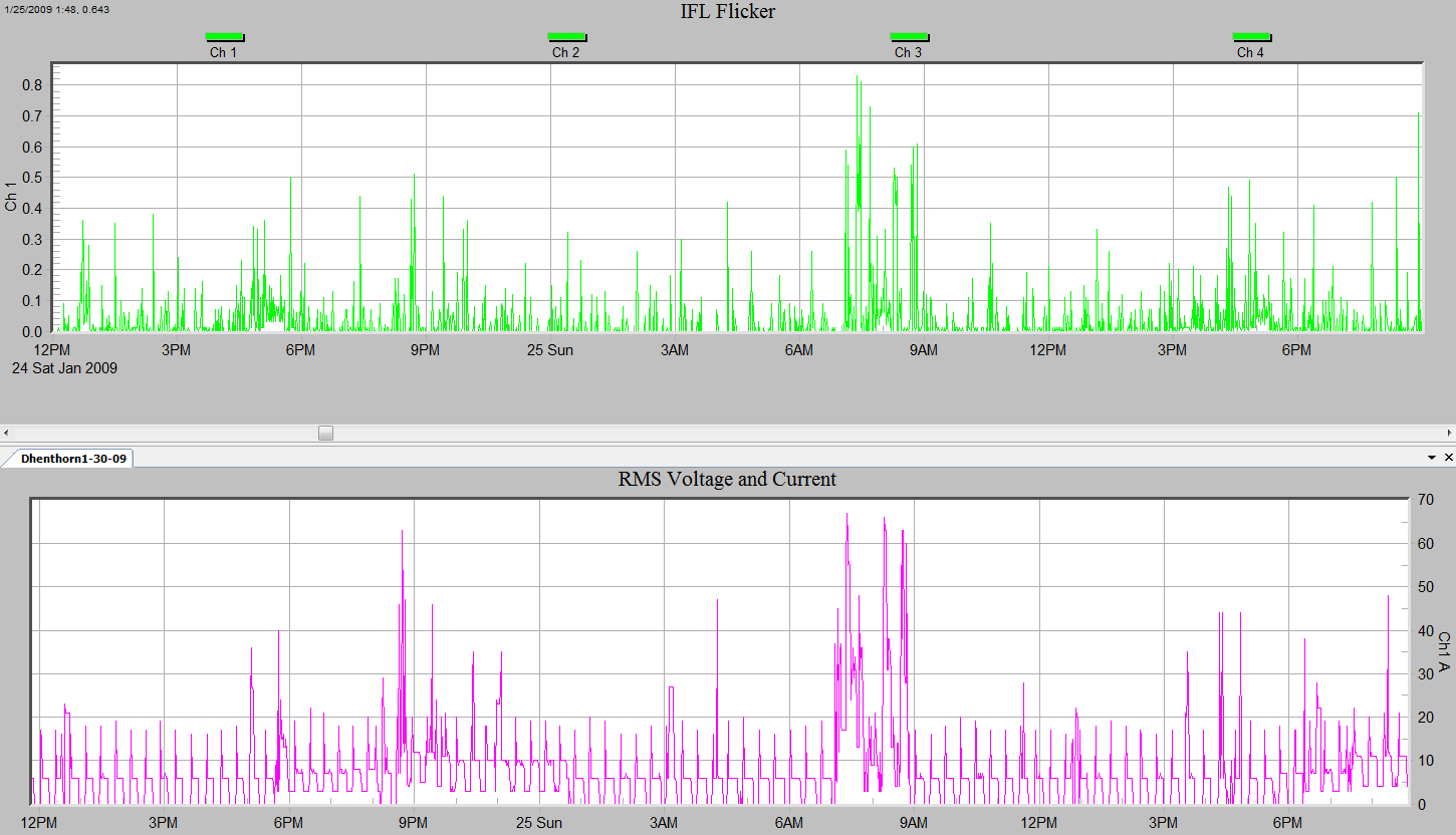
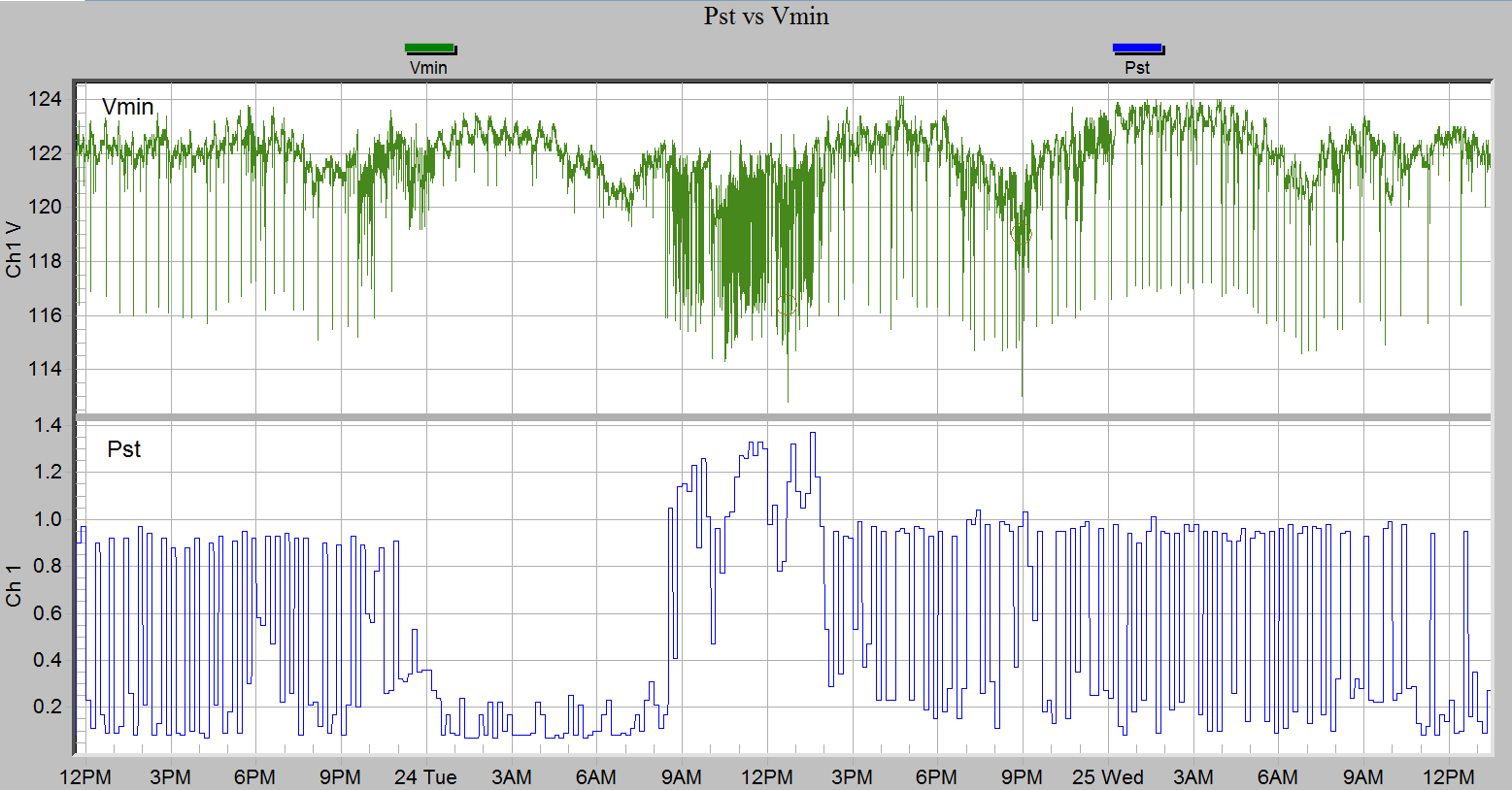
Both the severity of Flicker and the direction from the point of monitoring can be determined by recording the correct data. The severity of flicker is captured with a Pst (Perceptibility Short Term) interval graph while the direction from the point of monitoring is captured using voltage minimum, current maximum and IFL (Instantaneous Flicker Level) interval graphs. Refer to Figures 2 and 3. ProVision can be set up to capture each of these graphs in a single recording session via the Interval Graph tab when initializing a recorder. The Revolution, Guardian, and Eagle series (including the Eagle 120) all measure IFL and Pst flicker, and these stripcharts should be enabled in any recording where flicker is suspected. For more on recording Flicker download the paper “Strategies for Investigating Flicker”.

Flicker Limits

The engineering unit for instantaneous flicker is defined so that a value of 1.0 corresponds to the irritability threshold or borderline of irritability curve. Limits for flicker are based on a statistical analysis of samples of the Instantaneous Flicker Level (IFL) signal. These are dimensionless quantities (ΔV/V). They are designated as Pst (Percentile short term) which indicates the severity of the flicker on a short term basis of 10 minutes.

The formula for calculating Pst which indicates the severity of the flicker on a 10 minute basis is as follows:

Pst = √(0.0314P_0.1 + 0.0525P_1s + 0.0657P_3s + 0.28P_10s + 0.08P_50s)

Pst is typically used for short duration duty cycles, evaluated over 10 minute periods. The upper limit for Pst is 1.0.

One Plt can be calculated based on 12 successive Pst values.

The upper limit for Plt is 0.8.

• Useful for determining combined effect of several randomly operating loads (welders, motors)
• Also considers effects of flicker sources with long/variable duty cycles (arc furnaces)
• Typically evaluated over 12 Pst intervals – 12 x 10 min. = 2 hours

To establish immunity levels, subjective testing similar to what was conducted in establishing the GE flicker curves was carried out. Half of the people tested reported the flicker level was both visible and irritating when the Pst measurements were at 1.0 or above. Therefore flicker levels at 1.0 or above are generally considered as a potential problem.

IEEE 1453 Recommended Flicker Limits to Avoid Complaints

Compatibility Levels / Planning Levels

	Low, Medium V < 35 kV	Medium V 1 kV – 35 kV	High V < 230 kV	EHV > 35 kV
Pst	1.0	0.9	0.8
Plt	0.8	0.7	0.6

• Compatibility Level is chosen when a certain tolerable percentage of immunity-related problems may occur
• Planning Level is typically selected to be less than or equal to the compatibility level
• IEEE 1453 recommends using 95% probability level to determine compliance; where the connected load could exceed limits 5% of time and be in compliance
• 99% probability level is preferred
• Minimum assessment period of one week

Conclusion

1. The IEEE/IEC flicker measurement process, part of a power quality monitor, is designed for quick and thorough measurement of flicker.
2. The process accounts for all waveform shapes and frequencies.
3. The process was developed in Europe but was adapted into the IEEE Standard 1453 in 2005.
4. The signal chain is composed of filters and weighing “circuits” that compensate for light bulb characteristics and physiological characteristics such as the human eye and brain. The filters and weighing circuits develop a band of frequencies that the human eye is most sensitive.

The IEEE/IEC standards give a thorough signal chain for computing flicker. It was designed to handle any type of voltage variation that’s perceptible as light flicker, be repeatable among different PQ analyzers, and provide a quantitative time series representing the amount of flicker. PMI recorders such as the Revolution, Eagle/Eagle 120, and Guardian implement this standard, and present the data in graphical stripchart form. Understanding the reasoning behind the flicker standard and the details of the signal chain allows for a deeper understanding of what it’s measuring, and how to interpret the results.