Understanding Harmonics

Abstract

With the increase in nonlinear loads (VFDs, high efficiency heat pumps, electronic power supplies, etc.) and the reduction in excess distribution capacity, harmonic distortion is an increasingly common power quality issue. Most PQ equipment today can measure harmonics, but without a good understanding of what harmonics are, the numbers aren’t very helpful. Here the fundamental concepts behind harmonics are described.

The ideal voltage waveform produced by a rotating generator is a sine wave. A sine function can be expressed as:

where V_t is the value at time t, A is the amplitude (peak value), f is the frequency in Hertz, and φ is the phase angle in radians. Any sine function can be fully described by those three parameters: amplitude, frequency, and phase (see Figure 1). In an ideal 120V-nominal system, the utility voltage is sinusoidal, with A=120√2=167V, F = 60Hz, and φ=0 (although φ isn’t very meaningful without an absolute starting reference, or reference to another sine wave). A key property of a sine wave is that it’s periodic: V(t) = V(t+nP), where P is the period (1/frequency), and n is any integer. Each period (cycle) of the sine wave is identical to every other period.

Figure 1. Amplitude, frequency, and phase

Normally the only driving source in the distribution system is the utility voltage; this voltage sinusoid is the forcing function that all loads react to, by drawing current as determined by their load characteristics. With simple resistive loads, the instantaneous current drawn is exactly proportional to the voltage, and thus the current is a sine wave with the same frequency and phase shift, but (usually) different amplitude. With a mix of reactive loads, the total current is still a sinusoid with identical frequency, but the amplitude and phase angle may change from the voltage sine wave. Due to the special properties of the sine function, any linear system driven by a single sine wave will always result in an output of the same sine wave frequency, with no other distortion in the wave shape. Multiple linear loads produce sinusoidal currents that can be vector-added to determine the combined sine wave.

Nonlinear loads throw a monkey wrench into the system. Technically, a system F is nonlinear if it doesn’t obey the superposition principals for inputs x and y: 1. F(x+y) = F(x) + F(y), and 2. F(ax) = aF(x). In AC power systems, this means that a load is nonlinear if it produces a non-sinusoidal current waveform when driven by a voltage sine wave (or it produces one or more sine waves of different frequencies).

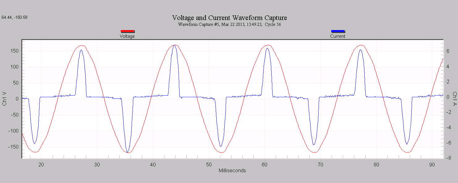
In general, a nonlinear load could theoretically produce any current waveform, even something completely unrelated to the driving voltage. Fortunately, most nonlinear loads aren’t as complex as that. Many are nonlinear only in that they draw current during just portions of the voltage sine wave. A simplified example circuit is shown in Figure 2. Here a diode rectifies the AC voltage, and a capacitor smoothes the rippled output into a mostly DC voltage. This DC is applied to the load, shown as a single resistor. This AC→DC conversion concept is found in most electronic power supplies, and is responsible for much of the harmonic current in today’s loads. The diode conducts only when the AC voltage on its left side is higher than the smoothed voltage (held up by the capacitor) on the right side. Figure 3 shows the voltage at the “Rectified DC” point, along with the original sine wave. The AC voltage is only higher than the rectified voltage for a small portion of the sine wave; this time period is known as the “conduction angle”.

Figure 2. Simplified electrical circuit

Figure 3. AC -->DC conversion” loading=”lazy”><figcaption>Figure 3. AC –>DC conversion</figcaption></figure>
<p>This load is nonlinear, as seen from the fact that the current drawn is not strictly proportional to the voltage at each point in the 60Hz sine waveform. It is periodic though – since it’s driven by a periodic forcing function; the resulting current waveform, while not sinusoidal, is still the same every cycle. Figure 4 shows the input voltage (red) and current (blue) waveforms from a real switching power supply. Here, the conduction angle is very small, and current is only drawn at the peaks of the voltage waveform. The current is not a sine wave shape, but it is periodic – it repeats with the same period as the driving voltage waveform.</p>
<figure><figcaption>Figure 4. Voltage and current waveforms from a switching power supply</figcaption></figure>
<p>Many, if not most nonlinear loads share this property. If driven by a voltage sine wave, the current waveform may be distorted, but it will have the same waveform shape every cycle. Fortunately, there is a powerful method of analysis for these waveforms – the Fourier Theorem. This theorem states that any periodic signal can be decomposed into a unique summation of pure sine waves, each with a certain amplitude, and phase, and whose frequencies are whole multiples of the base frequency (the inverse of the waveform period).</p>
<p>Mathematically, this can be written as:</p>
<p>Here, x(t) is an arbitrary periodic signal, and is equal to a summation of sine waves with the kth sine having amplitude A<sub>k</sub>, phase φ<sub>k</sub>, and frequency equal to k/P, where P is the fundamental period. In other words, any distorted, but periodic waveform may be decomposed into a series of pure sine waves at multiples of the fundamental frequency, each with different amplitudes and phase angles.</p>
<p>In a normal distribution system, the fundamental frequency is that of the voltage driving source, nominally 60Hz. A distorted waveform may be decomposed into a combination of sine waves with multiples of that frequency; these are known as harmonics. The harmonic number indicates the frequency multiple – e.g. the 1st harmonic (the fundamental) is 60Hz, the 2nd is 120Hz, 3rd is 180 Hz, etc. The Fourier theorem states that any distorted, but periodic, wave shape has a unique decomposition of a 60Hz sine wave, plus a 120Hz sine wave, plus a 180Hz sine, etc. In most AC power systems, the even harmonics are mostly zero in amplitude due to cancellations in 3 phase systems, and symmetries in most nonlinear load currents. In Figure 5, three harmonics, the fundamental, 3rd, and 5th are shown individually, then added together as an example of how pure sine waves can combine to form a distorted waveform.</p>
<figure>
<img decoding= — Figure 5. Pure sine waves can combine to form a distorted waveform.

A complete Fourier analysis includes a magnitude and phase angle for each harmonic. In most cases, the magnitude is much more important than the phase. The magnitude determines the size, and thus the importance of each harmonic to the overall distortion. The phase angle is usually not of interest, although in some specialized cases it can be used to help determine harmonic power flow direction, and the source of harmonic currents.

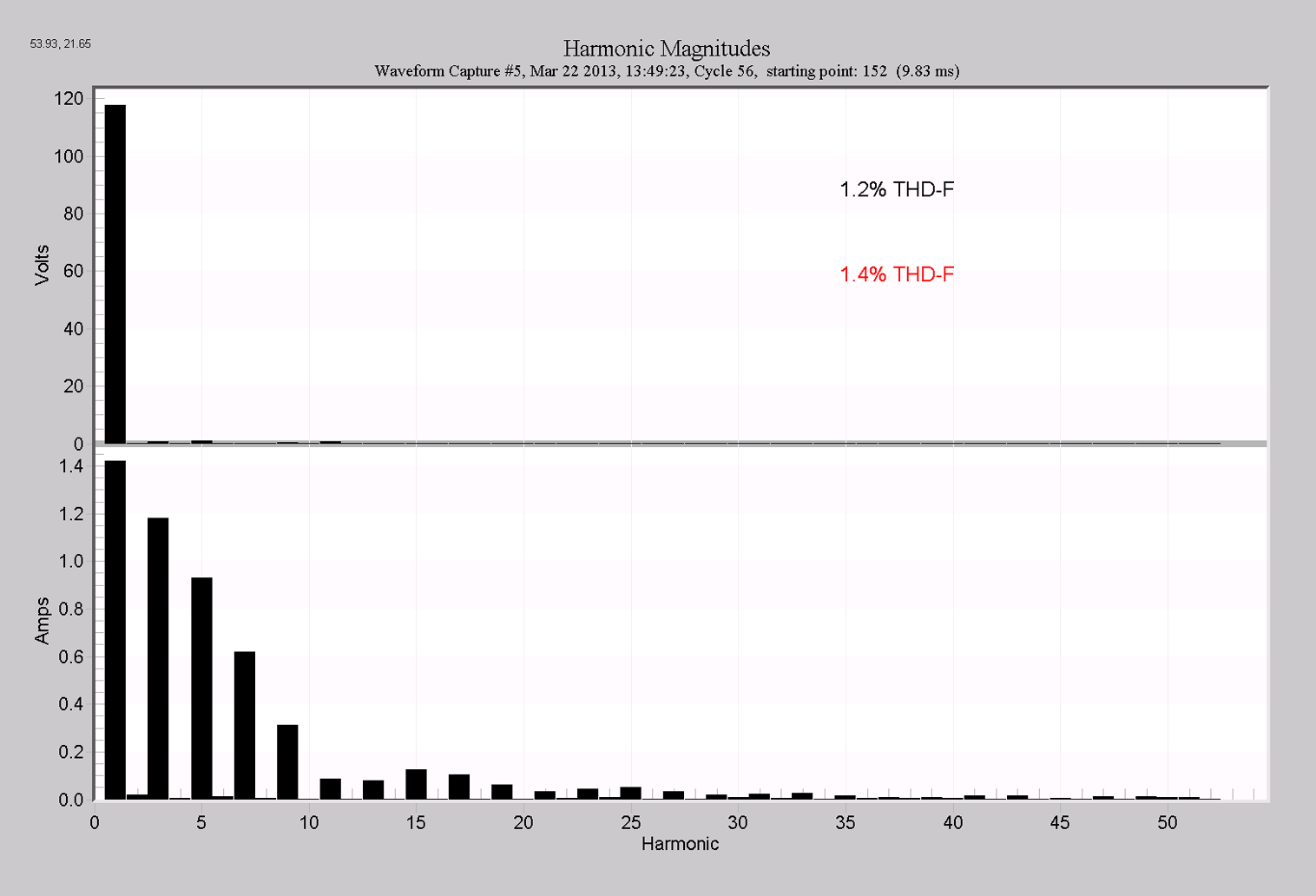
In Figure 6, the ProVision harmonic decomposition for the waveforms in Figure 4 is graphed. The harmonic number is on the x-axis, and magnitude on the y-axis. We can see that the voltage waveform is not very distorted – the main component is the 120V fundamental; the others are at most one pixel tall in the graph.

The current is much more distorted, and consequently the harmonic levels are much higher. The third harmonic is nearly as tall as the fundamental, and the 5th, 7th, and 9th are very significant.

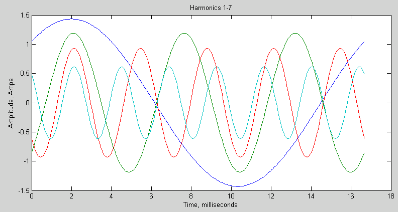
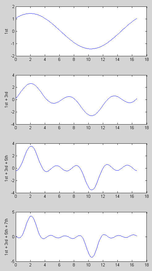
To illustrate how those harmonics truly do represent the original waveform in Figure 4, the first seven odd harmonics from Figure 6 are shown in Figure 7. Here harmonics 1, 3, 5, and 7 are plotted together, with their actual amplitudes and phase shifts from the harmonic decomposition. In Figure 8, the first harmonic is shown at the top, then the 1st plus the 3rd, then 1+3+5, and finally 1+3+5+7. The composite waveform gets closer in shape to the original in Figure 4 as we add more harmonics, and it’s approaching the final shape already with just four of them. In fact, with just 8 numbers (amplitude and phase of four harmonics), the waveform of Figure 4 is mostly characterized. Adding the higher harmonics gets the combined waveform closer and closer to the original one, but as the higher harmonic amplitudes get smaller, their addition has less of an effect. Generally the harmonics above the 31st are too small to matter, and often just the harmonics at the 15th and below are dominant.

Figure 7. Harmonics 1, 3, 5, and 7 plotted together

Given the sinusoidal voltage driving function, and generally linear nature of the distribution network (e.g. wiring, transformers, and capacitor banks) apart from the loads themselves, most complex current waveforms decompose into a relatively compact set of a few dominant harmonics.

Although the current waveform in Figure 4 (or any periodic waveform) can be described as a summation of harmonics, that doesn’t mean the physical generation of the waveform involved multiple sine waves. That current pulse was due to a narrow conduction angle in an electronic switching power supply, and the envelope of the current during the small conduction angle itself follows the voltage sine wave shape. Regardless of how the waveform was physically generated, it can still be treated mathematically as a summation of harmonics, and is identical to a waveform that was. In particular, passing a distorted waveform through a filter or trap tuned to a harmonic will effectively subtract that harmonic from the waveform mathematically, due to the superposition principle. If a heavily distorted waveform must be “cleaned up”, it’s sometimes possible to find a dominant harmonic, and filter that out. The result will be less distorted.

The distribution system’s frequency response is far from flat, due to power factor correction capacitors, and the many inductive loads. These capacitors and inductors form resonances in the system response, and accentuate or attenuate harmonics. A frequency breakdown of complex waveforms can be helpful in predicting interactions with resonances, or discovering the resonances themselves.

In more complex situations, a distorted waveform may not be periodic with a 1/60Hz period, or periodic at all. In these cases, a waveform is not the summation of a series of harmonics, and an even more powerful tool is required – interharmonics. The whitepaper Defining Interharmonics discusses this concept. Usually interharmonics arise when there are other AC sources present – either distribution generation, or AC→DC→AC systems (e.g. variable frequency drive systems).

A harmonic analysis is a powerful way to decompose a complex, distorted waveform into simpler parts. Due to the nature of most nonlinear loads, most distorted waveforms are characterized by a small set of harmonics, which can be analyzed separately. Most PMI recorders can measure and record harmonics, and ProVision can compute harmonics from any captured waveform.