Abstract
Capture high-speed, high-voltage transients with the Revolution and Vision, using the optional transient capture system. Transient capture uses 1 MHz sampling for voltage, giving a 1 microsecond sample window, and includes a +/- 5000 Volt full scale on all voltage inputs. Designed for capturing disturbances originating from lightning strikes, switch closures, and high frequency resonances, transient capture catches events missed by traditional waveform capture, or cycle-based recording.
Most power quality recorders sample the voltage and current waveforms at up to 256 samples per power line cycle. This is considered high speed sampling for traditional RMS and power measurements, and even harmonics – it’s enough speed to measure up to the 128th harmonic, in theory. That sampling rate equates to roughly 65 microseconds per sample (1/(256 x 60) = 65.1 us), or 1.4 degrees (360/256 = 1.4). The PMI Eagle and Vip recorders use this sampling rate, and with 600V RMS full-scale inputs, they have enough range to measure over +/- 1000 Volts on an instantaneous sample basis.
Although most power quality events are easily measured with the above sampling characteristics, a small, but important set are not. Transients caused by high-speed events such as lightning strikes, arcing from switches (e.g. cap bank or tap changer operations), or excitation of local high-frequency resonances can occur in just hundreds or even tens of microseconds. The peak value of such transients can exceed thousands of volts, even if just for a few microseconds.
The Revolution and Vision recorders feature optional transient capture capability. This includes a voltage input range of +/-5000 Volts (that is, 10 kV peak-peak) on the same voltage inputs used for regular monitoring – no special hookup or alternate inputs are needed. This is over 5 times the input range of a traditional 600V RMS input. The voltage is sampled at 1 MHz on each channel, which gives 1 microsecond per sample. This is 65 times more resolution than regular waveform capture, or equivalent to 8320th harmonic! The current inputs also have high speed sampling – 250 kHz on each channel, or 4 microseconds per sample.
These high speed data samples are fed into the transient capture triggering and recording systems on the Revolution and Vision. The high speed data is then filtered and downsampled to form the 256 samples/cycle data streams used by regular waveform capture, RMS and power calculations, etc.
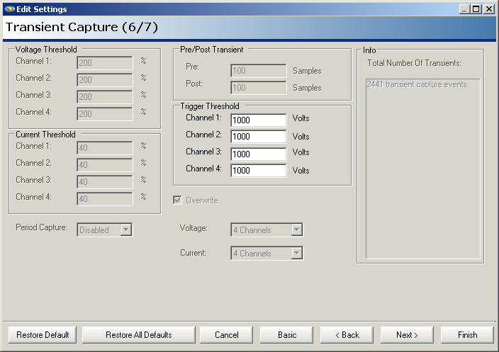
The setup for transient capture recording is on the 6th page of the ProVision settings wizard. Transient capture is triggered by exceeding the peak voltage threshold on any voltage channel. Each voltage channel has a separate threshold value. In the example shown in Figure 1, the threshold is 1000V. With this value, if the instantaneous voltage (e.g. one or more 1 microsecond samples) exceeds 1000V, a transient capture is triggered. The threshold is bipolar: if the voltage falls below -1000V, a transient is also triggered. Setting a voltage threshold to zero, or to a value over 5000V will disable triggering on that channel.
When adjusting the transient threshold, the first principle to keep in mind is to set the value higher than the peak of the highest expected RMS value. For example, if monitoring on a 120V circuit, the voltage will rise to 1.41 x 120V = 167V every half-cycle. If the transient capture threshold is set lower than 167V, it will trigger on every normal half cycle, overwriting any actual transients. A rough rule of thumb is to set it at least 50% higher than the highest nominal peak. For example, on a 120V circuit, the peak is 167V, so 50% higher would be roughly 250V. On a 480V delta, this works out to roughly 1000V. These would be suggested minimum values – instead of 50%, 100% or higher may be appropriate. As shown in Figure 1, the default value of 1000V is high enough to avoid trigger on the AC sine wave at 480V, but low enough to still be useful even on 120V circuits.
When a transient is triggered, a 1000 sample transient waveform is captured for all voltage and current channels. With a 1 MHz sampling rate, 1000 samples is a 1 millisecond time period. This is long enough to capture most high speed transients; but if the event still exceeds a threshold after 1 millisecond, another transient capture will trigger immediately.
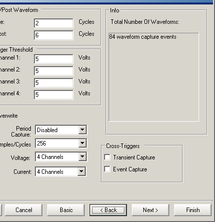
Another important transient setting is actually a waveform capture setting – waveform capture cross-triggering. In the Cross-Triggers section of the Waveform Capture wizard page, a checkbox for “Transient Capture” is shown (Figure 2). If this is checked, a transient capture trigger will also trigger a waveform capture. The waveform capture will use the slower 256 samples/cycle data stream, but will show multiple power line cycles, and make reveal clues about the source of the transient. This is especially useful for transients caused by tap changers or capacitor bank operations, since these have characteristic waveform signatures, and may not trigger a waveform capture themselves in certain situations.
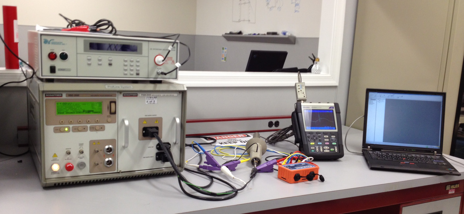
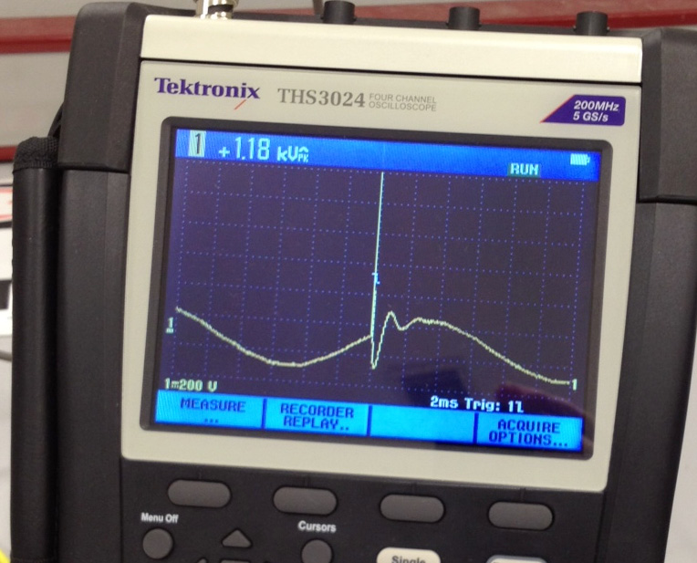
To illustrate the transient capture option, and contrast it with waveform capture, a standard test pulse was recorded as shown in Figure 3. In this test setup, a Schaffner NSG 2050 pulse generator was used to produce a standard 1.2/50 us pulse, as described in IEC 61000-4-5. This pulse shape is designed to simulate high-voltage transients commonly found in CAT III or CAT IV locations. It’s defined by a fast 1.2 microsecond rise time, and a 50 microsecond decay time, with a 2 ohm source impedance. The Revolution was connected to 120VAC through the pulse generator, and the generator configured to deliver a 1 kV transient superimposed on the 120VAC waveform. The generator allows for adjustment of the peak voltage, as well as the point on the 60Hz waveform to start the pulse. A Tektronix THS3024 oscilloscope was used to independently verify the pulse output as shown in Figure 4.
The relative speed of the peak transient compared to the 60Hz AC waveform can be seen in the oscilloscope displays.
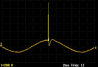
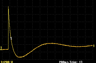
The first trace, as shown in Figure 5, shows the transient at the peak of the 60Hz waveform. The vertical scale is 200V/division, and the 1000V peak is clearly seen with the high-speed sampling of the scope (actually around 1100V, including the 60Hz waveform). The next trace (Figure 6) shows a zoomed in view, at 200 us microseconds per horizontal division. The main transient is much less than a single division – under 150 microseconds, as expected with a nominal 1.2 us rise time, and 50 us decay. The actual pulse rise and fall times are a bit longer, due to loading of the pulse generator. The longer multi-division undershoot and decay is due to slower resonances between the Schaffner internal capacitors and stray circuit capacitance. Note that the peak of the sine curve can just be seen in this zoomed view.
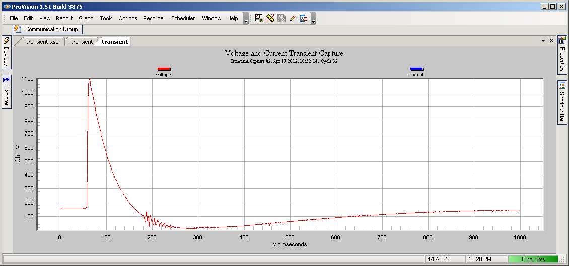
In Figure 7, we see a peak to over 1100V (the nominal 1 kV pulse plus the peak of the 60Hz waveform, followed by the slower decay. Zooming in, and enabling data point markers (Figure 8), shows the very fast rise time – the full voltage is developed in just a few microseconds.
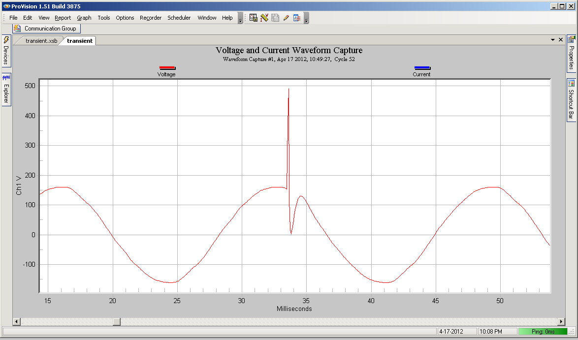
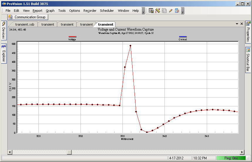
As shown in Figure 8, the waveform capture display in ProVision from the Revolution mirrors the slower scope trace. However, due to the slower 65 us sample width (from 256 samples/cycle), the peak voltage of the transient is not fully realized. The peak is just under 500V in the waveform capture recording – this is due to the very fast 1-2 microsecond peak being averaged into a 65 us standard waveform capture sample.
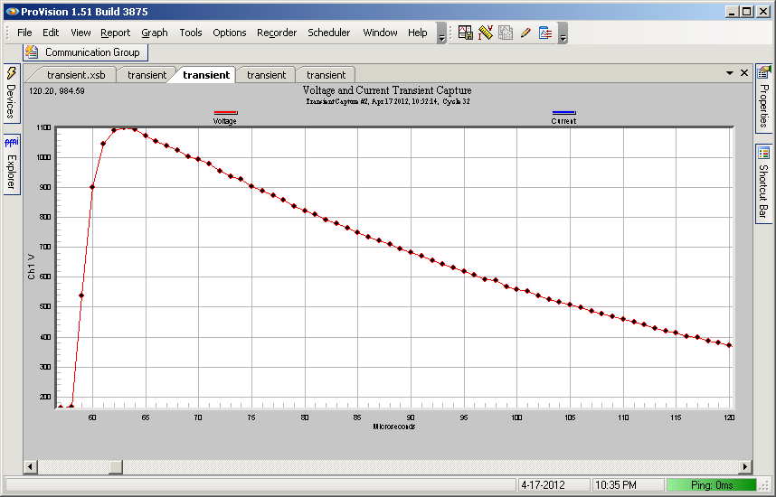
Since transient capture sampling is 65 times faster than regular waveform capture, 65 transient capture points occupy the same time period as a single waveform capture point. In the plot shown in Figure 9, 65 transient capture points are shown. This entire sequence is averaged into a single data point in regular waveform capture. The entire transient is over in just a few data points in the waveform capture graph (Figure 10). However, it is useful to see the entire 60Hz waveform, and the slower undershoot and recovery is well characterized by the waveform capture.
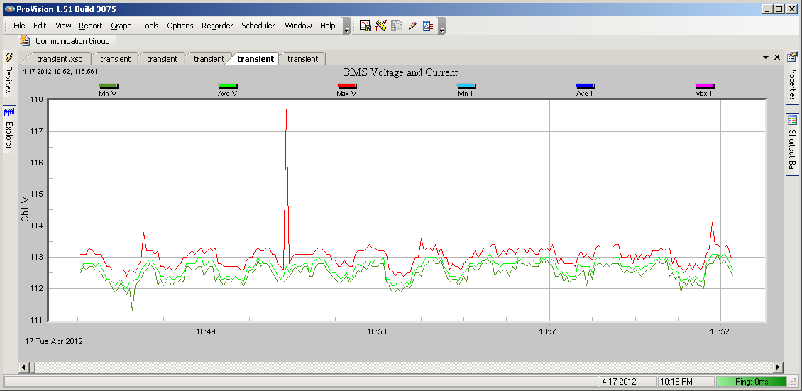
On an RMS voltage basis as shown in Figure 11 (top), the transient is almost invisible. In this graph, the waveform data is graphed using a sliding half-cycle RMS voltage window. The RMS voltage increased from 113.5V to 117.7V – a four volt increase, from a 1000V transient.
As shown in Figure 11 (bottom), the event also looks relatively innocuous in the RMS Voltage stripchart. Although clearly visible in this relatively clean graph, a spike to 118V would normally appear harmless.
The high-speed nature of these transients implies a high-frequency, wide bandwidth characteristic. Since the power line system attenuates high frequencies, these transients are typically localized – the further away from the source, the lower the peak voltage, and slower the transient becomes. Consequently, it’s important to place the recorder as close as possible either to the service entrance, to the most sensitive equipment, or to the suspected transient source, depending on the monitoring goals. For example, if a particular piece of equipment is experiencing unexplained resets or failures, monitoring right at the equipment disconnect is best. If the voltage feed to a customer is being assessed, monitoring at the service entrance, or point of common coupling is best. Or, if a capacitor bank or voltage regulator is suspected of generating switch noise or arcing during operation, monitor as close as possible to it. A distance of a few hundred feet can significantly reduce the peak voltage of a high frequency transient, so the recorder location is important in characterizing these events.
Conclusion
Transient capture in the Revolution and Vision is essential if high-speed, high-voltage events must be recorded and accurately measured. Although waveform capture data can indicate a possible transient problem, high speed sampling is needed to see the true voltage peak. Although real transient problems aren’t as common as voltage sags, swells, flicker, and other garden-variety PQ issues, when they do arise, only high speed sampling can show the true picture.
