Abstract

A harmonic analysis is a powerful method for analyzing waveform distortion, given the periodic nature of most nonlinear loads. Steady-state harmonic tools are sometimes extended for use with waveform events such as oscillatory transients, where the underlying assumptions behind the analysis are no longer true. Although a useful technique, it’s important to understand the differences between true steady-state harmonics, and the “harmonic” values generated from a transient waveform analysis to avoid drawing false conclusions.

Harmonic Basics

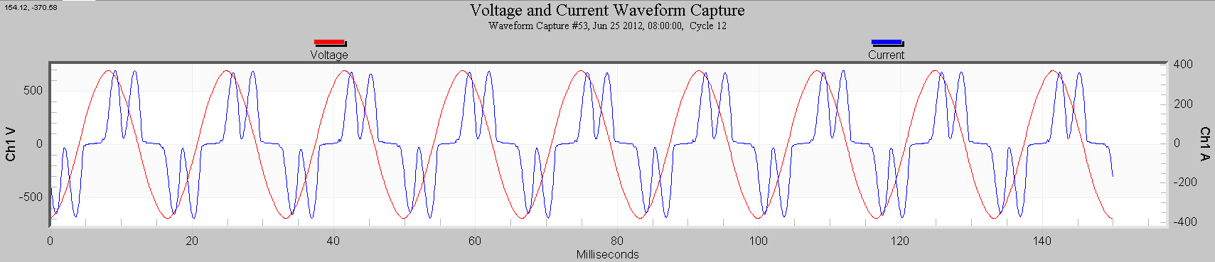
A harmonic analysis provides a similar tool for complex waveforms. In a harmonic decomposition, a non-sinusoidal periodic voltage or current waveform is broken down into a summation of pure sine waves, each with a frequency that is a whole multiple of the line frequency. In many cases it’s simpler to then analyze the harmonics rather than the original complex waveform. For example, consider the voltage and current waveforms in Figure 1. The blue trace is a typical phase current waveform from a 6-pulse Variable Frequency Drive (VFD). The current waveform is definitely not a pure 60 Hz sine wave, but it is periodic – the distorted shape repeats essentially unchanged in every 60 Hz cycle. For a VFD, the current pulses are produced in this consistent fashion due to diode conduction in the 3-phase bridge rectifier block – each branch of diodes conducts for a portion of the waveform as the phase-to-phase voltage changes in each branch. The underlying AC voltage sine wave drives this conduction pattern, and thus it repeats as the voltage itself repeats at the line frequency. The current waveforms of many nonlinear loads are driven by the AC voltage waveform, and thus are also periodic – the waveform distortion is the same with each driving AC voltage cycle. This property is why a harmonic analysis is useful for a wide variety of nonlinear loads. Loads where the nonlinearity is not periodic, such as arc welders, rock crushers, etc. are not amenable to a harmonic analysis.

With a consistent, periodic distortion, the Fourier theorem states there is a unique combination of sine waves that add up on a point-by-point basis to equal the original waveform, and that only sine waves at multiples of the line frequency are needed to do this. The advantage of using a harmonic decomposition is that many complex waveforms seen in the field can be represented by just a handful of harmonic values, reducing a complex shape into just a few quantities. This reduction in complexity is similar to how the RMS value can be used to simplify some calculations instead of using the entire waveform.

Steady-State Example

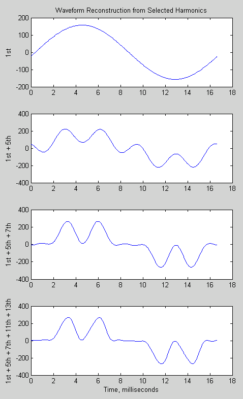
The particular wave shape from a VFD in Figure 1 produces harmonics of order n according to n = 6k ± 1, where k = 1,2,3, … and n is the harmonic number. This gives the fundamental (1st harmonic), then pairs of significant harmonics – 5th and 7th, 11th and 13th, 17th and 19th, etc. with the rest mostly zero. In practice, the first two pairs, 5th/7th and 11th/13th are the most important. A harmonic analysis was performed on a typical cycle from Figure 1, and as expected, these pairs are the largest. The decomposition gives amplitudes for each harmonic needed to reconstruct the waveform, and only a handful are needed. In Figure 2, a reconstructed waveform is shown as more harmonics from the decomposition are added together. The top plot shows just the fundamental, which of course appears as a pure sine wave. The second plot shows just the 1st and 5th harmonics, and the rough pulse shape of the original in Figure 1 can already be discerned. In the third plot, the 7th harmonic is added (1st, 5th, and 7th together), and here the reconstructed waveform already looks very similar to the original, with just three sine waves – the fundamental, and the first VFD pair. Finally, the bottom plot shows the waveform with the additional 11th/13th pair of harmonics included, showing that the point of diminishing returns has already been reached in terms of adding more harmonics to the reconstruction to reproduce the original waveform.

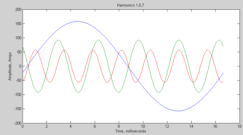
The 1st, 5th, and 7th harmonics are plotted individually in Figure 3, with their correct scale as per the harmonic analysis of Figure 1. These three sine waves, added together point-by-point, give the third waveform in Figure 2 – a very close match to the original in Figure 1. Thus, three sine magnitudes capture the essence of the complex waveshape from this VFD. Instead of further analyzing a complex shape, these three harmonic components may be analyzed further.

The current distortion here is a steady-state phenomenon – the VFD current is driven by the repetitive voltage sine wave. This characteristic is essential to the entire harmonic analysis concept, and is what guarantees a unique and complete harmonic breakdown of a waveform. This steady state nature is one reason for the IEEE 519 recommendation of at least 3 second averages for harmonic studies, and also longer 10 minute averages. Stripchart logging of average harmonic readings provide the raw data needed for steady-state analysis as per IEEE 519.

Oscillatory Transient Example

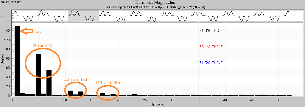
However, ProVision and other tools also provide a harmonic analysis of captured waveform data. In Figure 4, the VFD current waveform from Figure 1 is plotted in ProVision in the harmonic analysis window (Graph, Harmonic Analysis, Magnitudes), with voltages and the other phase currents removed for clarity. At the top, the entire waveform capture is graphed, with a gray analysis rectangle available. ProVision computes the harmonics of the cycle data inside this gray rectangle; this rectangle may be moved by the user. The dominant harmonics are the 1st, then 5th and 7th, and then the smaller pairs of 11th/13th, 17th/19th, as expected for the VFD waveshape. Since each cycle is very similar to the others, moving the gray data rectangle within this waveform capture doesn’t change the result much.

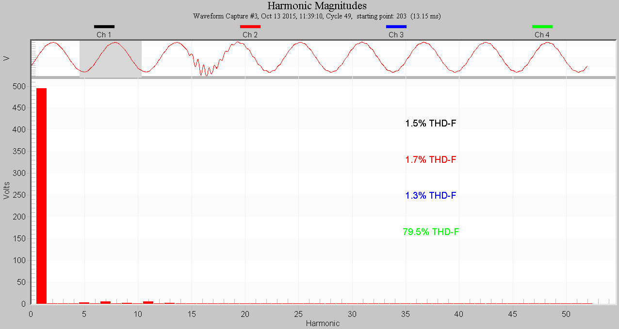
But what happens for a waveform where the distortion is not periodic? A harmonic analysis can still be useful, and ProVision can be used to compute the harmonic levels, but how are they meaningful if the assumption of periodicity is not met? In Figure 5, an oscillatory transient is graphed in the ProVision harmonic analysis tool. The gray selection rectangle is moved to cover a “normal” cycle, before the disturbance. This cycle looks much like all the others, so the traditional harmonic technique is valid. The overall distortion is low at 1.7%, and the harmonics themselves are very low compared to the fundamental, with the 7th and 11th being most dominant.

In Figure 6, the analysis rectangle has been moved to cover the oscillatory transient (circled in orange). The harmonic picture is much different now, with a lump of “harmonics” clustered around the 11th. The 10th and 12th harmonics are also elevated. But are these really valid, since the assumption of a periodic distortion is not met?

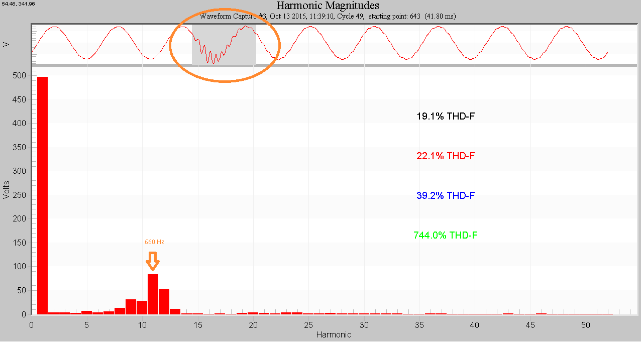
Strictly speaking, if no line frequency period is assumed for the distortion, the Fourier analysis doesn’t yield harmonics, but gives a spectral energy breakdown of the signal. Instead of referring to the fundamental, 5th harmonic, etc. the output of the algorithm should be interpreted as a set of frequency “bins” that cover the spectrum from DC to the half the sampling frequency. The x-axis for the bar chart shown in Figure 6 can be interpreted as frequency instead of harmonic number, where the 1st harmonic is 60 Hz, the 5th is 60×5 = 300 Hz, etc. The bars represent the amount of signal energy contained in each frequency bin, which in this analysis method is 60 Hz wide. For example, the 11th harmonic shown in the graph represents the energy in the signal centered around 660 Hz, i.e. 630 Hz to 690 Hz.

Here the concept of a fundamental, or multiples of that frequency (harmonics), even/odd harmonic patterns etc. do not apply. The plot in Figure 6 is interpreted purely as spectral display with 60 Hz resolution, plotted from 60 Hz to 3060 Hz (51×60). The readings cannot be considered harmonics since the waveform distortion does not repeat with each power line cycle. The THD reading is not really meaningful here either.

There is still a physical meaning to the spectral plot though, and useful information in it. A disturbance like the oscillatory transient in Figure 6 is very common, often caused by capacitor bank switching. The initial switch impulse excites a resonance formed by the cap bank and load inductance. This resonance produces a ringing waveform superimposed on the base 60 Hz sine wave, as seen in Figure 6, whose frequency depends on the capacitance and inductance. The distortion is sinusoidal, so a frequency-based spectral analysis still paints a useful picture. Here the dominant frequency is roughly 660 Hz (11×60), easily seen in Figure 6. The spectral analysis again allows for a simple representation of a complex waveform – 60 Hz sine wave plus 660 Hz ringing, with the caveat that this doesn’t imply a steady-state condition.

The peak at 660 Hz, and the lower, but still high region around that frequency don’t represent steady state harmonic levels. The peak is the ringing frequency, and the region around the peak represents windowing effects from the analysis technique, along with the fact that the ringing itself is damped and doesn’t persist throughout the analysis window. Knowing the resonance frequency allows for mitigation with a tuned filter, or further capacitance/inductance work to possibly detune the network.

The same analysis tool is used in Figures 5 and 6, but the interpretation is much different. With repetitive waveform disturbances, true harmonics are present, and the bar chart represents these harmonics. These harmonics can compactly describe typical patterns of distortion such as the one shown here for the 6-pulse VFD. With one-shot disturbances, the graph represents a generic frequency spectrum with 60 Hz resolution. Areas of high magnitude in the spectrum don’t represent steady state harmonics, but instead describe transient phenomena that typically persist for less than one 60 Hz cycle. Due to the reactive nature of the power line, and abrupt switching excitation, ringing transients are very common and are well suited for display with a spectral graph.

Conclusion

A spectral analysis is useful for both steady-state and transient waveforms. Although the mechanics for data analysis and presentation are the same, the interpretation and conclusions that can be made are much different. The background behind both types are given here, along with examples of each. A good understanding of the principles behind the method is important for extracting as much information as possible from the data while not drawing false conclusions.