Abstract
The combination of Canvass and Boomerangs strategically placed in a distribution system allows for a unique system-wide analysis of voltage trends. Analyzing voltage data from multiple locations in parallel reveals events originating from transmission lines. The local responses to transmission events can also be identified. Carrying the process further allows for a separation of secondary voltage events from distribution level events for a specific customer.
Superposition
A typical simplified electrical network consists of a single transmission line (“upstream”) that feeds several substations (“downstream”). Each substation has its own distribution network, consisting of multiple circuits, each of which has multiple customers, each of which has multiple loads. When a load is switched on, the current it draws flows through the complete path from the transmission line, through the substation, the distribution line, and down to the load. Voltage drop across any length of wire in that path is seen by all other loads that tap off the same path. The further upstream, the less the voltage varies from a given load change, since the total impedance is smaller.
From a voltage source point of view, all the endpoints are essentially connected in parallel. If there were no loads switched on, there would be no voltage drop along the line (since no current is flowing), the voltage at the end of each circuit would be identical, and proportionally follow any voltage shifts from the transmission line.
Due to the superposition principle, both the series and parallel effects happen at once, and are additive (ignoring any nonlinearities and feedback effects). This means that any voltage variation sourced from the transmission line will appear to all downstream devices. Voltage sags from loads inside a distribution network will not be as severe upstream, due to the lower source impedance further upstream. By overlaying voltage traces from devices in different locations, the type of event (transmission vs. distribution) can often be determined.
Spotting Transmission Events
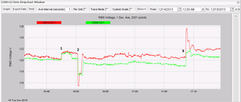
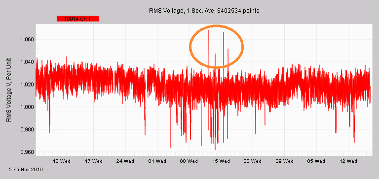
An example of a transmission event is shown in Figure 1. Here two Boomerang voltage traces are shown, covering a span of roughly 35 minutes. These two are 20 miles apart, on different substations (actually different utilities). They’re both fed from the same 230kV transmission line though (from a 3rd larger utility). In this case, a 230kV capacitor bank had an issue which caused several multi-second events. First we see a small 1% voltage swell (at 1), followed by a 4% drop (at 2), then 15 minutes later, a short 5% swell (at 3). The sag and swell only lasted for roughly one minute. The short voltage swell was characteristic of this cap bank problem, and from a longer graph (3 months, Figure 2) it’s clear that it only happened a few times over a few days – the problem was fixed quickly. Voltage swells can indicate cap bank switching issues, and the same voltage increase on multiple devices on different circuits indicates an upstream source.
Checking Regulator Responses
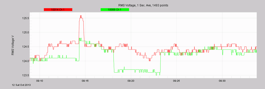
Often local voltage regulators will automatically adjust the line voltage in response to a step change in voltage. With Boomerang strategically located through a system, these regulator actions can be checked easily. For example, in Figure 3 a step increase in voltage appears on both Boomerangs (same two from previous figures, on different circuits), as marked by the black arrow. Within 1 minute, the regulator on the red trace compensates, leaving the voltage just about 0.1V lower (on a 120V basis) than before, as marked by the first orange arrow. The regulator on the green trace waits about 5 minutes, then makes a tap adjustment that results in a lower voltage than before. It’s apparently not pleased with the result – 5 minutes after that, it makes a new adjustment, leaving the voltage just a slight bit higher than the start (rightmost orange arrow).
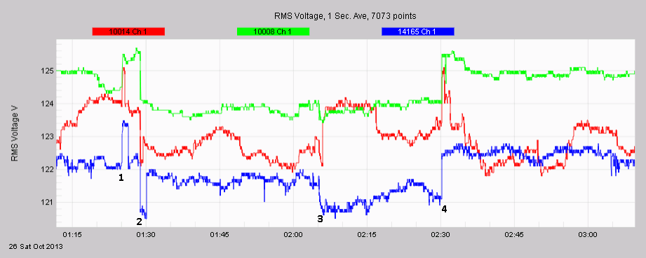
A more complex case is shown in Figure 4. Here, we have the same two Boomerangs, plus a Revolution (blue trace), located roughly midway between the two geographically (different substations). Four transmission line events are shown, numbered 1 through 4. At 1, each device saw a 1V voltage swell. The red Boomerang’s local voltage regulator again responded quickly, dropping the voltage back within a minute. The regulator for the blue trace responded next, after about 2.5 minutes. As shown in the previous figure, the green Boomerang’s regulator is slower to respond, and before it did here, another transmission line event happened at 2. Here the voltage dropped to just below the starting point, before 1. The red and blue Boomerangs’ regulators responded again, with their same characteristic delays.
A half hour later, at 3, the transmission voltage drops again by around 0.5V. The green and blue Boomerang regulators don’t respond, but the fast red one does, boosting the voltage by almost 2V. Five minutes later it backs off, lowering the voltage by 1V. Finally, at 4, the transmission line voltage jumps up 1.5V, then drifts down 0.5V over the next couple of minutes. Again, the red Boomerang’s regulator is quick to respond, actually adjusting twice in 3 minutes.
What can be learned from these three Boomerangs, all seeing the same transmission line events? The red Boomerang’s regulator is very fast to respond to voltage changes, making 6 adjustments. It’s not only fast, but also responds to small changes. The blue Boomerang’s regulator is slower, and not as “twitchy”, making 2 changes. Finally, the green Boomerang’s regulator is slowest (as seen in previous figures), and didn’t even adjust at all here. Its final voltage was also the closest to the starting voltage, despite not making any adjustments. The red Boomerang’s regulator is possibly set to make adjustments too often, resulting in increased wear and tear, and more voltage flicker for customers.
Boomerang Placement
To best characterize a distribution system with Boomerangs, two strategies can be used. First, to track what’s coming in from transmission, it’s helpful to have some Boomerangs along the transmission line. E.g. if 10 substations are fed from a single line, one Boomerang per substation would allow tracking voltage events as they vary down the line. Since the substation is the lowest impedance point on the distribution circuit, placing a Boomerang there provides the most separation between transmission events and local load-induced voltage sags.
Second, to characterize the distribution system itself, locate at least one Boomerang per circuit coming from each substation. The end of the line is often used for low voltage monitoring to meet regulatory minimum voltage requirements, but a mid-point can be better for overall monitoring, especially just after the first voltage regulator. Here “mid-point” would be the electrical midpoint, roughly past 50% of the circuit load. Ideally, a monitor would be installed at the substation, just past each regulator, and at the end of the line for each circuit. A compromise is to outfit one representative circuit fully, and use fewer monitoring points on other circuits from the same substation, possibly just one per circuit, but at similar locations (e.g. midpoint of circuit, end of line, or just past a regulator). If the load is mostly residential (i.e. mostly single-phase Boomerangs), it’s helpful to place one Boomerang on each phase somewhere along the circuit. By using the Virtual 3 Phase feature in Canvass, three single-phase Boomerangs can be combined to show voltage unbalance.
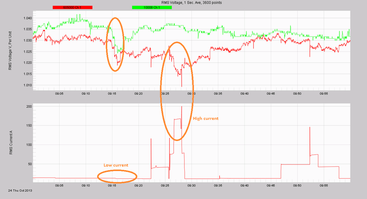
For large loads, it’s helpful to have current monitoring. In Figure 5, voltage traces for two Boomerangs are shown on the top graph, and the load current for the red Boomerang is shown in the lower graph. Two voltage sags are present. In the first sag, the voltage sags about 1% in about a minute for both Boomerangs. The sag origin must be upstream, since they both see the same excursion. About 18 minutes later, the red Boomerang shows a similar sag, but with no corresponding change on the other device. This sag source must be downstream of the green Boomerang, but upstream (or at) the red Boomerang. A quick view of the current trace for the red Boomerang shows the current increasing at the same time as the sag (confirmed by the quick current spike at the end matching the quick voltage sag) – the load right at this Boomerang is causing the sag. This is especially useful for circuits where a few large industrial loads dominate the circuit.
Conclusion
With strategic placement of Boomerangs, and Canvass graphing that shows multiple devices on a single graph, voltage events can be separated into transmission vs. distribution root causes. The distribution response to upstream changes can be characterized by watching for regulator and cap-bank changes that occur.
