Abstract
The RMS value is used to quantify the overall “size” of a waveform with a single number. By extension, harmonic amplitudes can be used to describe a complex waveform with just a few non-zero values. Understanding the relationship between an RMS value, harmonic amplitudes, and the total harmonic distortion (THD) of a waveform allows for a faster and more effective power quality investigation when faced with voltage or current distortion problems.
Brief Review of RMS Definition
RMS stands for Root Mean Square, which is exactly descriptive of the mathematical concept: take the square root of the mean of the sum of the squares of each element in a series:
where there are N samples in a 60 Hz period of a voltage or current waveform, x.
The RMS measurement is a means of calculating the magnitude of an arbitrary, but periodic waveform. It is also important to remember that the instantaneous value at any point in the time domain of an AC waveform can vary quite significantly – another important reason for calculating the RMS value of each point in the time-domain series of a single cycle of a waveform. For more background on RMS values, see the whitepaper Understanding RMS Measurements.
Harmonics
Every distorted, periodic waveform has a unique harmonic decomposition. What this means is that there is a combination of “harmonics” (sine waves with frequencies that are integer multiples of the 60Hz fundamental frequency) of various amplitudes and phases that can be added together point by point mathematically to form the original waveform. In many cases, a distorted waveform is more easily analyzed by examining the harmonic breakdown rather than the raw waveform itself. Those harmonic amplitudes RMS add to the overall RMS value of the original waveform. Note, too, that in general, the waveform is not physically created by a process of individual harmonics being summed together. Rather, the distortions in a waveform (the harmonics) are due to instantaneous load characteristics at varying points in the waveform. Even so, every periodic waveform can be represented by a unique combination of harmonics.
The harmonic decomposition of a waveform can be thought of as just a convenient mathematical tool for looking at the different “elements” within a waveform. It can be compared to the unique prime factorization for any whole number (e.g. 12 = 2 × 2 × 3).
Parseval’s Theorem
In its most fundamental form, Parseval’s Theorem demonstrates that the RMS value includes each individual harmonic magnitude in its calculation. From an energy standpoint, it states that the “energy” in a waveform when computed in the time domain (with raw waveform samples) is equal to the “energy” as computed in the frequency domain (with harmonics). Thus, each harmonic contributes to the RMS value. In fact the RMS value is itself an RMS sum of the harmonics.
Parseval’s Theorem is defined as follows:
RMS from waveform = RMS from harmonics
What this is stating mathematically is that the sum of the squares of the individual harmonic magnitudes (in the frequency domain) is exactly equal to the mean of the sum of the squares of each point in the time-domain. This is where the RMS time-domain and frequency domain equivalence comes from.
Effects of RMS Value on THD (and Vice Versa)
THD (Total Harmonic Distortion) is a measure that expresses the percentage of a waveform’s magnitude that is comprised of harmonic (non-fundamental) frequencies. There are two different THD methods: THD_RMS and THD_F where THD_RMS is the total harmonic distortion as a percentage of the RMS value and THD_F is the total harmonic distortion as a percentage of the fundamental magnitude. Mathematically, they are defined as follows:
THD_F = (√(Σ hn²) / h1) × 100%
where THD_F is the THD expressed as a percentage of the Fundamental, F is the magnitude of the fundamental and hn is the magnitude of the nth harmonic, and
THD_RMS = (√(Σ hn²) / XRMS) × 100%
where THD_RMS is the THD expressed as a percentage of the RMS value of the waveform, hn is the nth harmonic, and XRMS is the RMS value.
Notice that when calculating the THD for each case that the numerator begins its series at n = 2 indicating that the fundamental harmonic is not included in the calculation.
Take special care to consider corner cases in these calculations as well. Since THD-F is a division with the magnitude of the fundamental frequency as the denominator, as the fundamental goes to zero, the THD goes to infinity. This could be seen in a neutral current waveform, where the 60Hz component cancels from the 3 phases, but harmonics remain. In this situation, the THD-F isn’t very meaningful.
The THD_RMS in this case will max out at 100%.
Observations
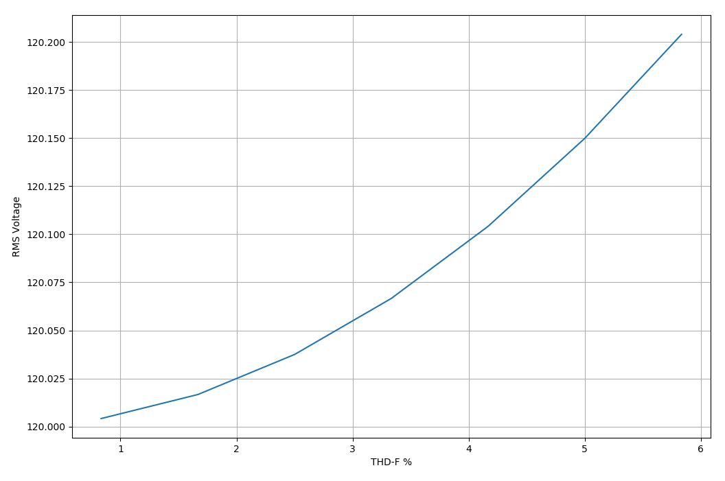
To illustrate the effect of increasing harmonics to the RMS and THD values, a waveform was constructed with a varying amount of harmonic distortion. Harmonic levels were increased gradually, and the resulting RMS and THD values computed. Figure 1 is a graph of THD-F vs RMS values for a voltage waveform (120V nominal), with harmonics increasing until THD-F is six percent. One of the first impressions is that it is clearly non-linear. While the increase in RMS is proportionally rising very rapidly, the raw increase in this particular case isn’t tremendous: from the run between 1% and 6% THD the RMS value increases by 0.3V or about 0.25%. Because the harmonics are an RMS sum, and also typically much smaller than the fundamental, the overall RMS value is not affected much, compared to the THD. Often, harmonics are subtracted from the waveform, rather than added, in the form of voltage drop due to nonlinear loads. In either case, the effect on the voltage RMS value is still relatively small compared to the THD. As shown in this example, a 6% THD (very high for voltage) is present with just a negligible 0.25% change in RMS value.
During the compilation of this paper some other interesting observations were made as regards the distribution of harmonics and the total harmonic distortion (THD). For instance, if the sum of the squares of all harmonic magnitudes is the same, regardless of their presence in a single harmonic or if they are spread over 50 harmonics or perhaps just over the even or odd harmonics, then the THD will be the same. For example, a 10V harmonic affects the THD and RMS value equally, regardless of whether it’s the 3rd or 5th (or any other) harmonic. And that makes mathematical sense, too. Consider the following examples.
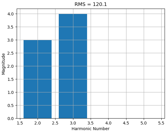
If a waveform has two harmonic components, the 2nd and the 3rd harmonics with the following magnitudes: h2 = 3 and h3 = 4 and the following is true:
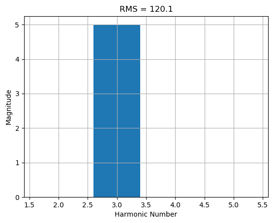
If, on the other hand, the waveform was comprised of a single harmonic (let’s call it the 3rd harmonic) with a magnitude of 5, then the following is true:
Assuming a fundamental of 120, then the THD_F for each is expressed as:
To tie it all together now, the question is: does the distribution of harmonic magnitudes – if the sum of their squares is equal regardless of distribution – affect the total RMS value for the waveform? Spoiler alert: it does not. As demonstrated above with Parseval’s Theorem, there is a time-domain and frequency-domain equivalence. This can be tested by generating waveforms with some harmonic distortions:
where Fmag is the magnitude of the fundamental, k is the kth harmonic, f is the frequency.
Figures 2 and 3 show how the sum of squares of harmonic magnitudes – as long as their sums are equal – produce the same RMS values (120.1V in this case). Figure 2 is comprised of a single harmonic (the 3rd harmonic) with a magnitude of 5V. Figure 3 shows a waveform that contains two harmonics, the 2nd and 3rd with respective harmonic magnitudes of 3V and 4V (Remember, 3² + 4² = 25 = 5²).
Also note that due to the square summation in Parseval’s theorem, a single large harmonic increases the RMS and THD values disproportionally compared to many smaller harmonics. As an extreme example, a 120V fundamental combined with a single 10V harmonic has a THD of 8.3% and RMS value of 120.42V. The same fundamental combined with 10 individual 1V harmonics has a THD of 2.6% and RMS value of 120.04V. Filtering a dominant harmonic may significantly improve the THD.
Conclusion
The equivalence between time- and frequency-domain analysis of waveforms, and its relationship to THD has been explored. The RMS (Root Mean Square) value does contain information regarding the waveform’s harmonic distortion. Additionally, it has been shown – thanks to Parseval’s Theorem – that the RMS value of a waveform can also be calculated by way of the frequency domain. As harmonics increase, the RMS value of a waveform increases slowly, while the THD increases at a significantly faster rate.
