Recommendations for Voltage Sags

Introduction

Voltage sag is one of the most common power quality problems. The consequences for not troubleshooting a voltage sag complaint isn’t the resulting damage that can be done to electrical equipment, but rather the resulting significant loss of revenue due to production line stoppages or process control interruptions. Some examples are presented here that cover various sources of voltage sag as well as how to select and configure a PQ recorder for data collection.

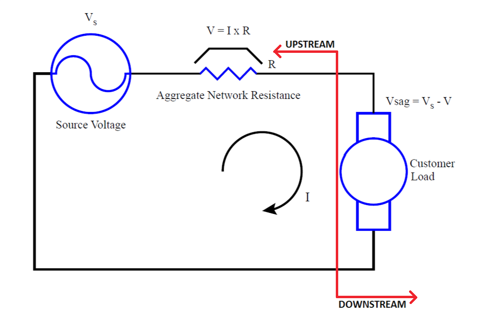
The most useful data to record are voltage and current intervals, and waveform captures. Current should be included in every recording session because the voltage data alone only tells part of the story. The current waveform (or signature) is representative of the customer load and can be used to separate out load issues (downstream) and power sourcing (upstream) issues.

Some Basics Before We Get Started

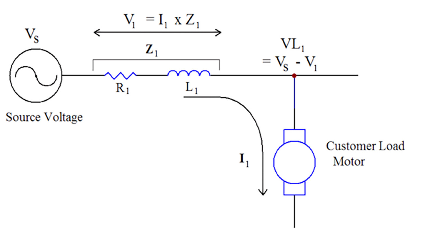
The first assumption that we can make about the power distribution system as shown in Figure 1 is that equivalent or aggregate system impedance looking “upstream” or back from the load is a constant over short durations such as hours or days. This will be more important in later discussions. In Figure 2, the customer load V_L1 sees source voltage V_s minus the voltage drop across the system impedance Z₁.

What’s an Acceptable Voltage Level?

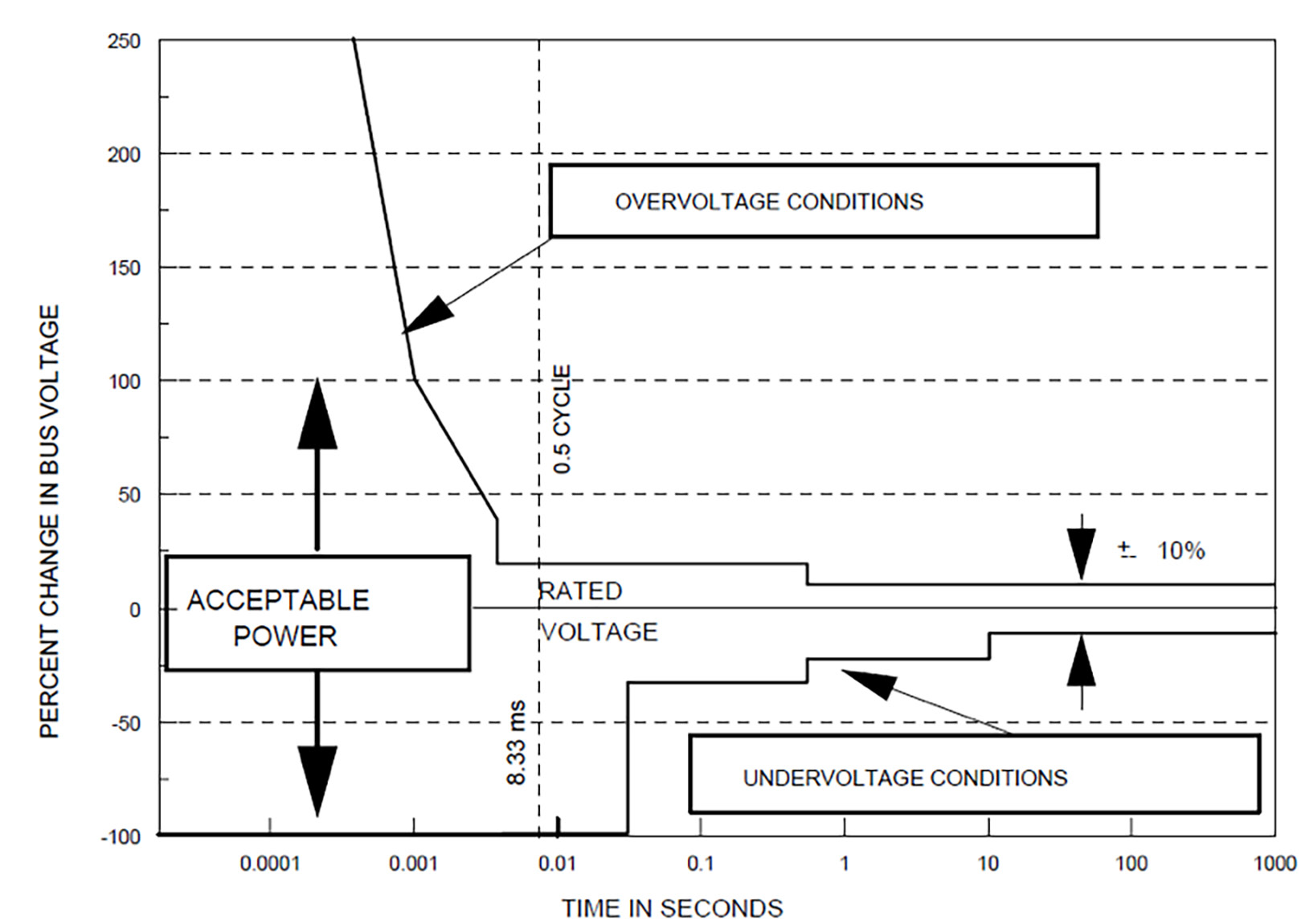
Unlike voltage dip which is considered a shorter term event under a half second, voltage sag is defined by IEEE 1159 as the remaining RMS voltage at the power frequency for durations as low as a half cycle up to 1 minute, after a decrease has been detected from 10 to 90% of nominal voltage. When a customer suspects that their equipment isn’t working properly due to excessive voltage sag, the ITIC power acceptability curve (newer version of the CBEMA curve) shown in Figure 3 gives the utility a metric based on percent from rated voltage for both under and overvoltage to determine if the sag is outside of acceptable limits. The y-axis is in percent deviation from nominal voltage and x-axis is in time, ranging from microseconds to steady state. For voltage sags, the applicable portion of the ITIC curve spans from 0.5 cycles to 1 minute. When the supply voltage stays inside the acceptable power area then the equipment should work as expected. If the voltage falls below the acceptable region (the sag region), equipment may malfunction, but should not be damaged. This is in contrast to voltage swells (increases in voltage), where exceedances past the curve could produce equipment damage.

Figure 3. ITIC Power Acceptability Curve

Like the ITIC curve in Figure 3, the semiconductor industry created SEMI F47-0706 in order to address service costs and increase tool reliability and uptime. Semiconductor processing equipment is especially vulnerable to voltage sag and requires a higher level of PQ, and will be harmonized with IEC 61000-4-34 which is the respective international voltage sag immunity standard. Figure 4 is the required voltage sag ride-through capability curve in which semiconductor processing, metrology, and automated test equipment must be designed and built to conform. The equipment must be able to continuously operate without interruption during conditions identified in the area above the defined solid black line.

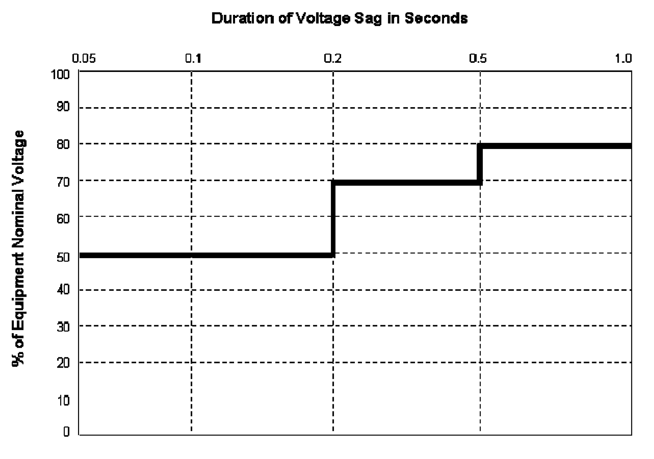
Figure 4. Required Semiconductor Equipment Voltage Sag Ride-Through Capability

Note: Equipment must continue to operate without interruption during voltage above the line.

General Sources of Voltage Sag

The list of voltage sag sources in Table 1 are common but certainly not complete.

Symptoms of Voltage Sag

Dimming of Lighting Systems
Relays and Contactors Drop Out
Equipment Resets or Not Working
Unreliable Data from Test Equipment
Variance in Production Rates
Variable Frequency Drives Resetting
UPS Operation

Getting Started

PMI’s Eagle, Guardian or Revolution recorders provide the ability to capture 1-cycle statistics for voltage sag analysis depending on sample speed and recording duration needed.

Next we need to select the following features for the recording:

Interval – Interval graphs are useful in seeing the big picture of captured recording. At a glance you can determine the max, min, average quantities and correlate them to a specific event. The interval graph can allow you to determine customer load issues vs. source issues. This correlation between utility voltage and load current is key for determining the root cause of a voltage sag.

Waveform Capture – Waveform capture is a useful tool to “zoom” in on the captured event and see what the cycle by cycle waveforms look like during the event. This allows you to determine the severity and what the cause of the event might have been.

RMS Capture – The RMS capture is a useful tool in determining the change of the RMS value over a fixed period of time. RMS capture is generated from the waveform capture samples for voltage and current. The RMS capture graph is a powerful method to visualize RMS changes in voltage and current, giving waveform-like detail without the inherent scaling issues of looking at raw sine waves.

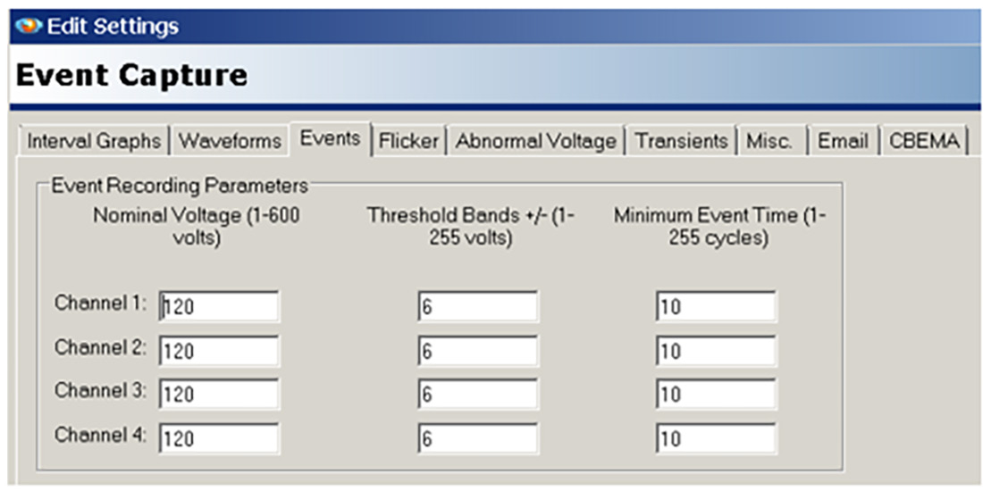
Event Change – Event change is similar to waveform capture, minus the raw waveforms. See setup screen in Figure 5.

Figure 5. Setting Up Event Change in ProVision

Interval Graph Examples

Interval Graph Example 1

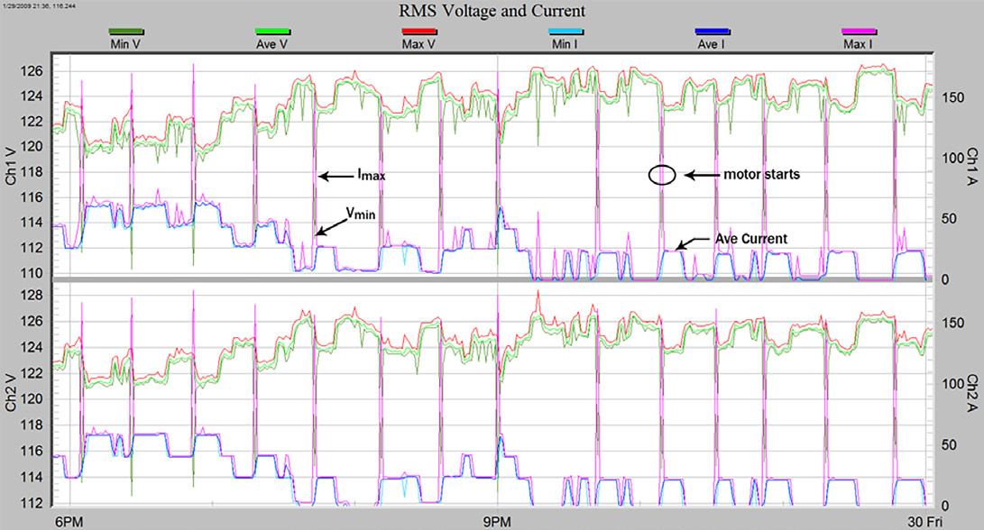
Figure 6. Voltage Sag Caused by Customer's Induction Motor — Figure 6. Voltage Sag Caused by Customer’s Induction Motor

Common loads such as a 4-pole induction motor can draw up to six times their normal running current. In Figure 6, voltage sag from an induction motor is noticeable on both Ch1 and Ch2 legs of approximately 10 volts. This information is gathered from the minimum (min) voltage interval point. The min voltage (dark green) is the lowest the voltage was measured in the given interval. Notice the max current (pink line) spikes about every 20 minutes on both legs at the same interval that the voltage sagged. This tells us two things; the load must be causing the sag, and it’s a 240V load. With further investigation we can conclude that the load is likely an induction motor.

Notice the inrush current and then the average running current. This type of load cycle is also typical of some heating systems.

Interval Graph Example 2

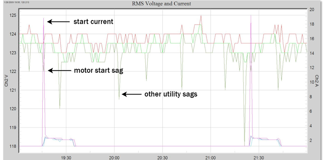
Figure 7. Voltage Sag Caused by Up & Downstream Loads

Unlike Figure 6, which results in a voltage change for each downstream load change, Figure 7 shows a 19A starting current resulting in a 1.5V voltage sag during a motor start but then deeper sags with little or no corresponding changes in current. Therefore, since the system impedance isn’t changing over this short period of time, the other voltage sags are a result of an upstream event, not customer load current.

Interval Graph Example 3

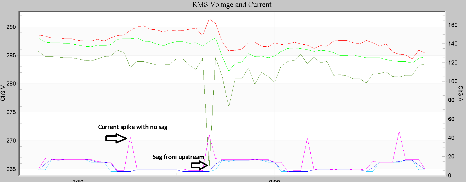
Figure 8. Apparent Voltage/Current Correlation, Unknown Case

A more complex example is shown in Figure 8. A 20A current spike shows no significant voltage sag, but a few minutes later a large voltage sag (15% drop) occurs during a similar 20A spike. Therefore the sag depth is related to the upstream system impedance which can be located with further data collection of loads in the system. Since the system impedance is relatively constant, if a 20A customer load spike didn’t cause a voltage sag at one point in a recording, it should not be able to cause one anywhere else in the recording. Thus, the deep voltage sag coincident with the second 20A spike is likely not caused by that spike. If it were, the other 20A spikes would cause similar sags.

Based on this short summary about voltage sag in single phase circuits, identifying the root cause isn’t always straightforward. However given the proper recording tools and training, the task of analyzing current and voltage data can be far less challenging and can prevent recurring financial losses.

This relationship may not hold in the presence of distributed generation. For example, a local photovoltaic system with an inverter on the same transformer’s secondary as the load may present a complex, or changing impedance.

Waveform Capture Example

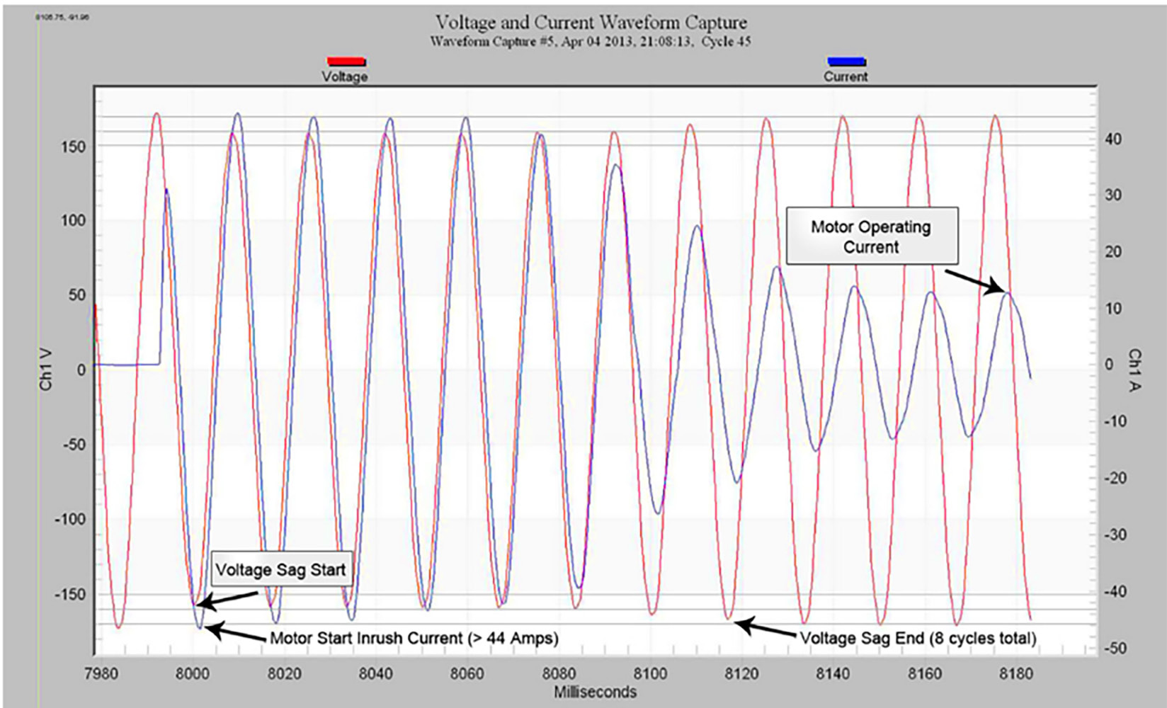
Figure 9. Voltage Sag Caused by a Different Induction Motor

Figure 9 shows a 120V induction motor which produces an inrush current of about four times the operating current. Notice that the voltage sag occurs from cycle 2 and continues to cycle 9.