Quantifying Residential Voltage Sags

Abstract

Voltage sag complaints are one of the most common in residential applications. Despite complaints, many residential voltage sags are not actually troublesome, or caused by the utility. Quantifying sag events and comparing them to industry-accepted thresholds helps separate true problems from situations where the customer is more sensitive than their equipment. Methods to quantify voltage sags and present this information in a clear manner are shown in this paper.

Voltage Sag Overview

A voltage sag is defined by IEEE 1159 as a “decrease in RMS voltage to between 0.1 and 0.9 pu at the power frequency for durations of 0.5 cycle to 1 minute.” For a 120V nominal, this corresponds to 12V to 108V. Most deep sags are caused by upstream faults that are quickly cleared by reclosers or distribution protection. Local loads, especially motor starts and other high inrush-current devices, can cause voltage sags, but these are often not as deep as utility faults. Poor connections or wiring problems can introduce extra resistance in a circuit, causing excessive voltage drop, and thus excessive sag as seen by downstream devices. Voltage events on a faster time scale are oscillatory or impulsive transients. Slower voltage events are interruptions, or regulation issues such as under- or over-voltage.

Many sags are visible to a residential customer as light “blinks,” but cause no problems with the loads themselves. Persistent visible sags are a possible flicker problem rather than a voltage incompatibility issue between the service voltage and the customer equipment. True problems from voltage sags usually involve equipment powering off or restarting — for example, a computer rebooting, heat pump restarting, air conditioner compressor shutting down, etc. Many electronic loads such as microwave ovens and TVs power off instead of restarting, and must be manually restarted. Equipment damage from isolated voltage sags is rarer, but overheating or reduced equipment life is possible from recurring deep sags that cause repeated inrush current. Residential voltage sags are generally simpler to analyze than commercial/industrial locations due to the single-phase service.

Spotting Voltage Sags

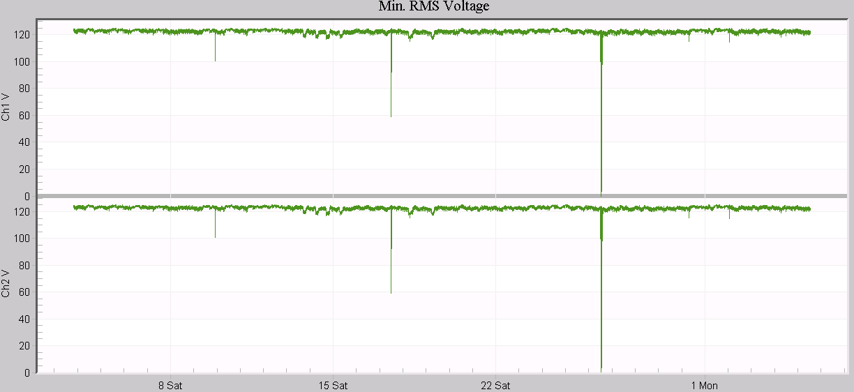
The default RMS Voltage and Current stripchart graph, while a good starting point for many investigations, contains more detail than is needed for initial voltage sag analysis. For sags, the 1 cycle minimum voltage is the most important trace. To graph just this data, choose Graph, RMS Interval, Overview, Minimum from the ProVision menu. This initial view is shown in Figure 1. The two dark green traces are the 1 cycle minimum values, recorded at the stripchart interval (1 minute in this data file). The average and maximum RMS values aren’t needed in this analysis so they’re not plotted. There are two major sags — one around 100V, one at 60V, along with one interruption.

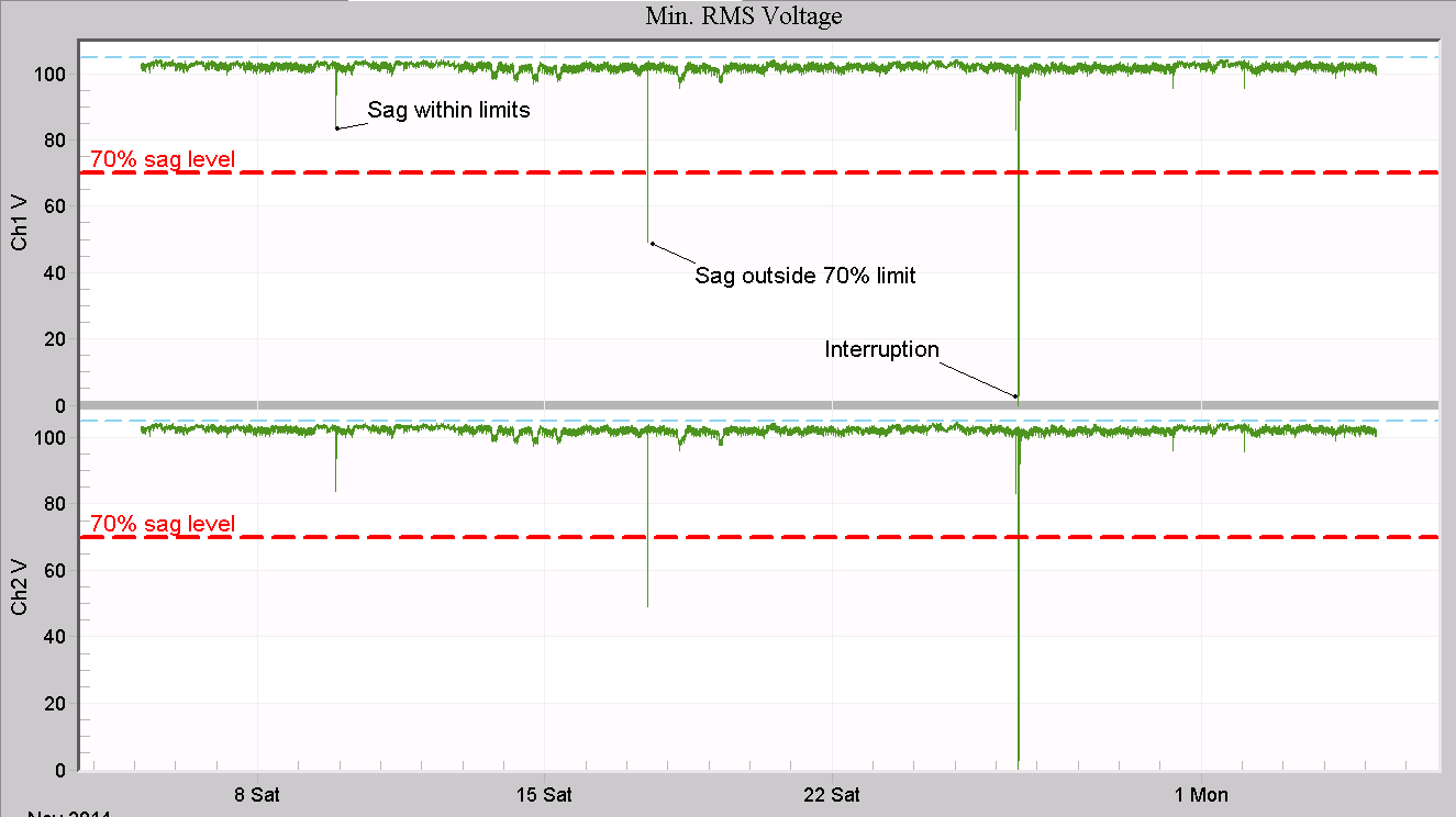
Figure 1. Raw 1 cycle min RMS voltage stripchart

An annotated version of the graph is shown in Figure 2. This presentation can be useful for sharing with customers. Some changes made from Figure 1:

Voltage data is scaled in per unit (x100), which helps a customer relate the level to a percentage, rather than a specific voltage value
Both y-axes scaled from 0 to 1.10 pu, to prevent auto scaling from magnifying a small sag
70% Sag depth marked with red dotted line, to visually indicate a go/no-go level for most sags
105% Upper limit marked with blue dashed line

This graph view makes it easier for a layman to understand whether sags on the graph are outside the limits — most events between the blue and red dotted lines are acceptable to most industry standards, as further discussed below. The per unit scaling (times 100) converts raw voltage values into percentage numbers, removing the unnecessary detail of the specific voltage nominal. In Figure 2, only one sag event approaches the red dashed threshold. The first sag is within the limit, and the right-most event is an interruption (voltage down to zero), not a voltage sag. The ProVision annotations have been used to mark these on the graph.

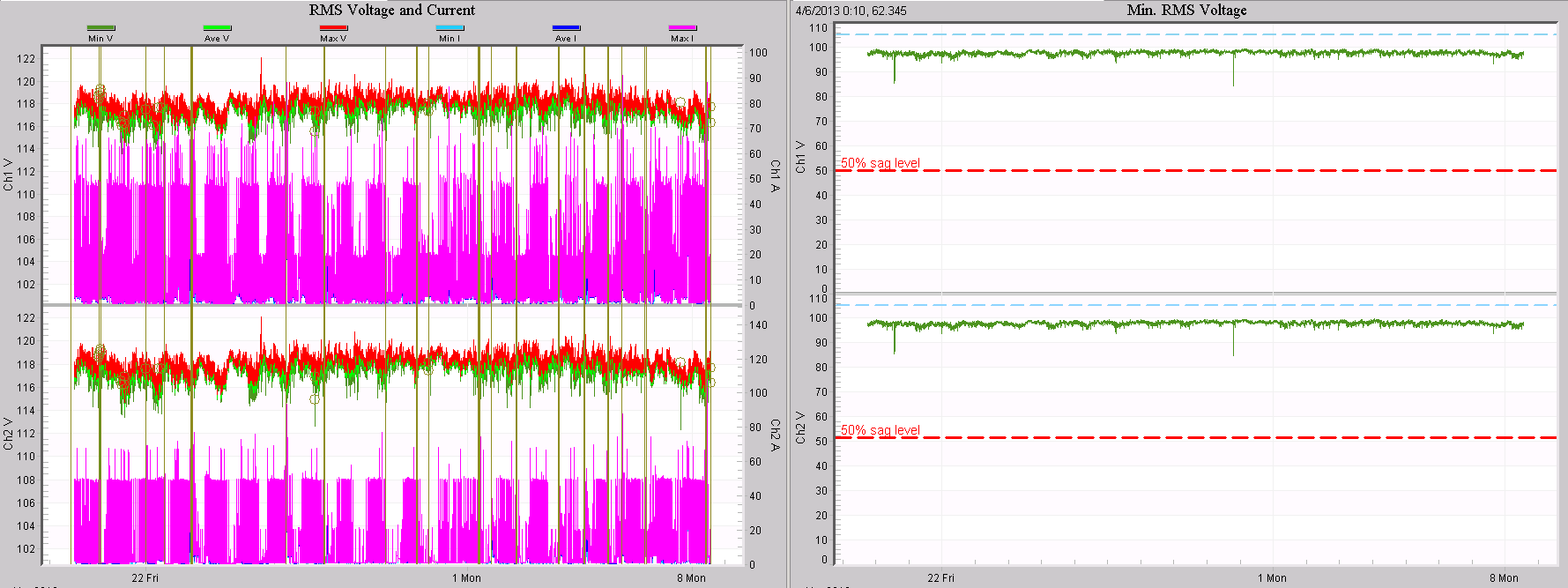
Figure 2. Annotated stripchart with sag limit and per unit scaling

A good “before and after” view is shown in Figure 3. On the left is the normal RMS Voltage and Current Stripchart graph, showing min/ave/max for voltage and current, waveform and event annotations, etc. On the right is the same data, but with just the minimum voltage traces, scaled and labeled as Figure 2. There are a couple of sags visible, but at 0.85 pu they are well within the limit of 50% used in this situation. The graph on the right is much easier to understand, especially for a non-technical customer if data must be shared.

Figure 3. Raw (left) RMS voltage and current stripchart, sag display (right)

Measuring Voltage Sags

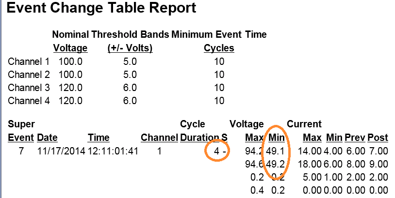
Voltage sags can be characterized by the sag depth and duration. The worst-case sag depth is easily seen in the stripchart due to the 1 cycle resolution, but the duration requires more data. Once a sag has been spotted in the stripchart, the next step is either waveform or event capture. The Event Capture report shows a tabular listing of all voltage events, with duration automatically calculated. Waveform capture shows a graphical view of the raw voltage waveform, and the duration can be measured with graphing tools. Event Captures are marked as small circles on stripchart traces; clicking on a circle will bring up the associated event. Figure 4 shows the event for the first sag in Figure 2. The duration in cycles here was 4, and the minimum voltage on each leg was 49V.

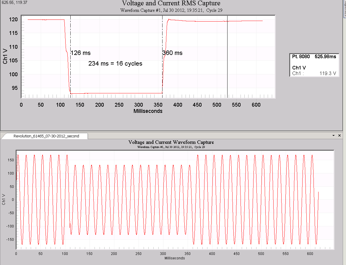
Figure 4. Event change capture of a sag event, with 4 cycle duration

A voltage sag waveform is shown in Figure 5. The bottom plot is the raw sinusoidal voltage waveform. The top plot is the RMS Capture graph, computed by ProVision with a sliding RMS computation window. For voltage sags, this RMS graph is easier to use than the raw waveform. The point table can be used to get exact millisecond times for the start and stop of the sag, and the difference divided by 16.66 ms to get the duration in cycles. In Figure 5, the start and stop are marked in ProVision with vertical annotations at 126 and 360 ms, giving a duration of 234 ms, or roughly 14 cycles.

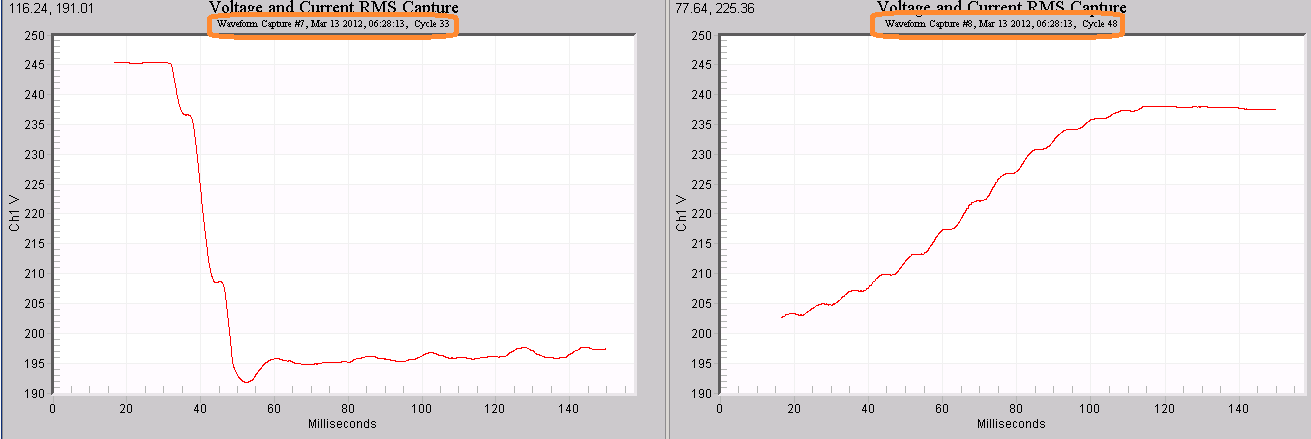
Figure 5. Measuring sag duration with RMS Capture

A long sag may generate two waveform captures — one at the start, and a separate one at the end. In this case the timestamps of each can be subtracted to determine the length. In Figure 6, two adjacent RMS captures show the start and stop of a voltage sag. Note the very steep beginning of the sag, followed by a more gradual end — typical of a motor start. The first waveform is triggered in cycle 33 of 6:28:13, and the second in cycle 48 of the same second. This gives a duration of 15 cycles, although there is at least one cycle of ambiguity due to the gradual return of the voltage. The waveform timestamps are at the top of the graph (circled in orange).

Figure 6. Measuring sag duration with a long sag that spans two waveform captures

Determining Sag Acceptability

In general, acceptable power quality is determined by the compatibility of the utility-delivered voltage with the customer equipment. In that sense, voltage sags that do not affect equipment operation are generally not a problem and do not need mitigation, even if they are noticeable by the customer (typically through isolated light flicker). There are several industry-standard guidelines for equipment operation and survivability for voltage excursions, including the CBEMA, ITIC, and SEMI-E10 curves, along with the SEMI F47 standard. These are standards for equipment manufacturers which specify regions of equipment operation, failure with no damage, and failure with equipment damage for various voltage events. There are differences in the details, but for voltage sags these standards generally indicate that equipment should continue to operate with sags down to 50% with durations up to 200 ms (12 cycles), 30% up to 500 ms (30 cycles), and 20% over 1 second. Many sags caused by upstream faults are cleared within 30 cycles, so 30% limit (0.7 pu) is a good starting point for sag acceptability, and 20% (0.80 pu) a good threshold which leaves some margin for low voltage conditions or longer sags. The 50% limit (0.50 pu) may be used when looking for short sags from upstream fast-acting system protection from faults.

One method for analysis is to mark the stripchart with a 70% or 80% threshold line. For any sags below that threshold, use waveform or event capture to determine the specific sag duration. If the duration exceeds the values above, the event likely falls outside the CBEMA/ITIC or SEMI-F47 window, and equipment misoperation (computer reset, heat pump cycling, etc.) is likely, and further investigation is probably needed. The Revolution and cell Guardian recorders can capture and display events directly on the ITIC curve, providing another mechanism for judging acceptability directly.

If a customer reports continued equipment problems even if the voltage sags appear to be within limits, then further investigation may be needed inside the premises itself. The voltage quality at the load may be much worse than at the service entrance. In this case, the service entrance data is key to determining whether mitigation is needed by the utility or the customer. If there is no actual equipment malfunction in a residential situation but a customer is noticing sags due to light flicker, then the problem may be more related to rapid voltage fluctuations rather than sags.

Conclusion

Voltage sags are a frequent source of customer complaints, often indirectly via reports of resetting computers, restarting heat pumps, and electronic equipment powering off. Quantifying sags at the service entrance is important to determine if there is an actual sag problem, and if so, whether the problem resides on the utility or customer side of the meter. Presentation of sag data to the customer may be required in cases where the source of the problem lies within the residence. Example graphs and an analysis strategy for analyzing voltage sags in residential situations has been presented.