Abstract

Previously, a method was shown to compute cycle event durations with one minute interval data and one-second timestamps from Significant Change data. In this whitepaper, a method is given that doesn’t require any data other than the one minute stripchart; this method results in a better duration estimate and allows for the calculation of event timestamps.

Event Duration

In Computing Event Duration with Interval Data, it was shown that a short event can shift the average in a stripchart interval enough to allow the calculation of the event duration. A real-world example of a motor start (from a water pump) was used. An Excel spreadsheet containing data from this example is available by clicking HERE. Before the motor starts, the average voltage is roughly constant at V_NL (no-load). During the event, the high motor-start current pulls the voltage to V_min, and after the sag, the loaded line voltage V_L is lower than the pre-sag voltage, due to the running current. The average voltage during the interval, V_ave, is a combination of V_NL, V_min, and V_L, with the exact value depending on precisely when the motor started in the interval, and how long the motor start lasted. Using N for the event duration (normalized so 1.00 = the interval period, and t for the fraction of time in the interval before the motor started, the expression allows for the computation of N. In the example from the earlier whitepaper, t = 39/60, V_NL=245.7, V_L= 238.4, V_ave=243.0, and V_min= 194.8, giving N = 12 cycles (after multiplying by 3600 to convert from normalized 1 minute intervals to cycles). Waveform captures from similar events in the data file show an event time of around 15 cycles, reasonably close agreement (and well within the 30 cycle CBEMA limit for an 80% sag).

However, a crucial piece of information was used from outside the stripchart: the Significant Change report was used to get the value for t. The event was time-stamped at 15:34:39, so the event happened 39 seconds into the 60 second interval. Without this one-second timestamp, the formula is unworkable. The formula is very sensitive to t – a resolution of one second is just tolerable. Using 38/60 or 40/60 (instead of the correct 39/60) gives durations of 2 or 22 cycles, respectively. What if we want a less sensitive method, or what if we don’t have any timestamps at all? Or what if we want both? There is a way.

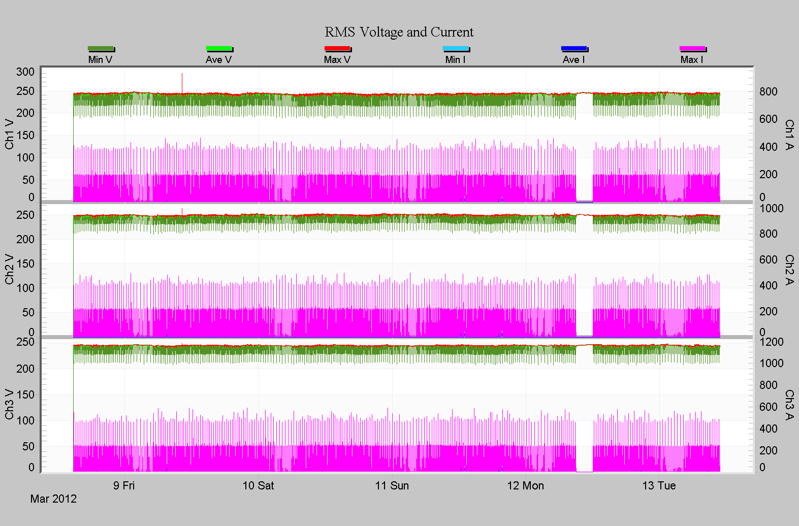
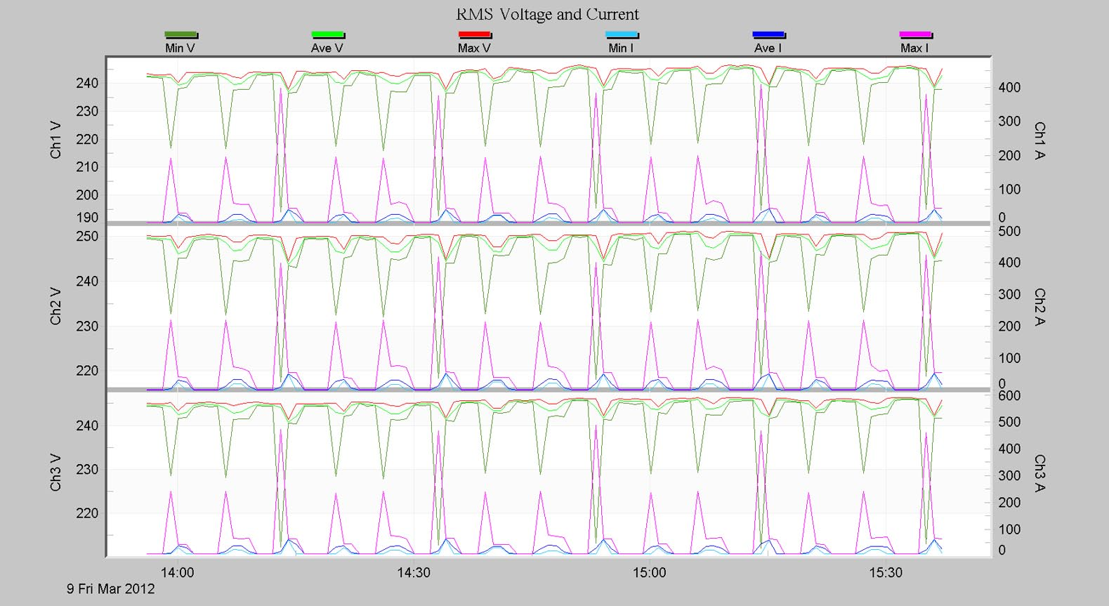
Looking at the interval data for the entire recording (Figure 1), we see that the pump started many times. Zooming in on a typical section, it’s clear that there are two operations happening (Figure 2). The primary event of interest is the 400A starting current that pulls the voltage to under 200V. A smaller motor appears to operate twice between each big motor start, with starting current around 200A, and sagging to 235V. Nothing much else happens in the interval data, except for these regular motor starts. That gives us a lot of clean data to work with, and lets us work with the interval stripchart data set, not just a single event.

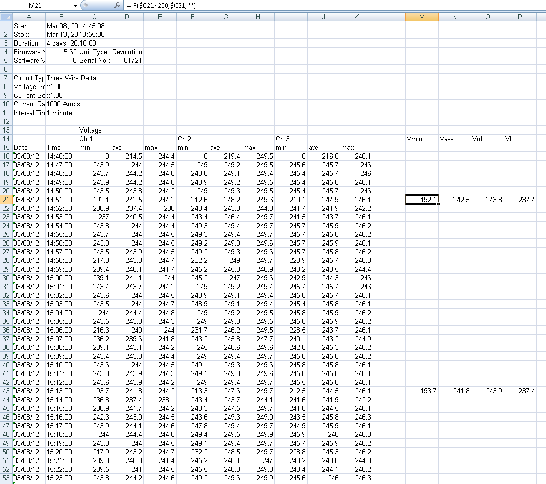
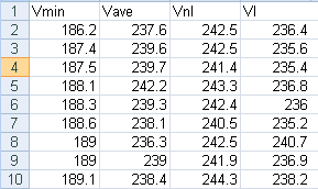
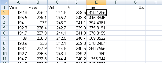
The interval data was exported to Excel (Report, Interval, RMS Voltage, then right-click and select “Export to Excel” in ProVision). An Excel spreadsheet containing this data is available HERE. Channel 4 was deleted, and columns were added for V_min, V_ave, V_nl, and V_l, as defined above (Figure 3). Conditional logic was used in Excel to only show values where V_min was under 200V, since this seems to separate the small motor from the large motor (the large motor sags to 194V, and the small one to just 220V). Since V_nl and V_l are pulled from rows before and after V_min, it’s easier to copy and paste these columns to a fresh worksheet, using Paste Special, Paste Value in Excel, removing any dependencies and pulling just the numbers themselves. The values can then be sorted, and the sags separate from the empty values (Figure 4). A count of these sags shows that the motor started 305 times during this recording – plenty of data to work with.

We will assume the motor starts were asynchronous to the recorder stripchart interval times, and randomly, uniformly distributed throughout the intervals. That is, each motor start occurred sometime randomly in a one minute interval, with each second between 0 and 60 being equally likely. With a uniform distribution over (0,60), the average value is 30 seconds, or t = 0.5. Using t = 0.5 for each sag event in the spreadsheet gives 305 values for the event duration, one for each sag. Since each individual event could happen anywhere in the interval, and very few actually were at 30 seconds, the event times for each individual sag are wildly inaccurate – ranging from +420 cycles to -264 cycles (see Figure 5 for the time column added, and sorted by time).

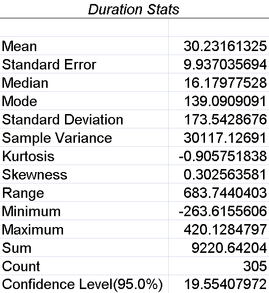
Since the sample average of a uniform random variable is the best estimator of the mean value, it follows from the linearity of the above equation for N that the sample average of N is an unbiased estimator for the actual sag duration. Hence, we can average all the individual sag durations, despite their wild values, and the average should be the best estimate for the actual duration. A closer look at the data is needed to make sure the assumptions are correct, but a quick averaging of all 305 values in column E of Figure 5 gives a value of 30.2 cycles, which is much closer than +420 or -264, but not very close to the expected 15 cycles (from known waveform data).

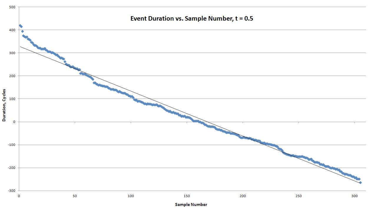
In Figure 6, the raw event durations for all 305 events, with t = 0.5 are shown in a scatter plot, with a best-fit line drawn. With a uniform distribution, ideally the durations would follow the line. Looking at the data, it appears that the first 50 or so points deviate from the line, and the rest would follow it closely. A more rigorous check is to take some basic statistics of the 305 durations. In Figure 7, the stats for column E of Figure 5 are shown (in Excel choose Data, Data Analysis, Descriptive Statistics). For a uniform distribution, the median should be close to the mean, the skew should be zero, and the kurtosis (a measure of the “peakedness”) should be -1.2. The numbers in Figure 7 don’t match very well, suggesting that not all 305 points are suitable. Possibly the outliers were from multiple events of different types in the same interval, or events that actually spanned two intervals.

Instead of using all 305 points, a better approach is to use a subset from the center of the dataset, avoiding outliers on either end. Taking 100 points from the middle of the data set and averaging the durations gives a value of 16 cycles – very close to the waveform capture result. Figure 8 shows the stats for the sample of 100 points. The mean, 15.6 (rounded to 16 cycles) is much closer to the median, the kurtosis is much closer to -1.2, and the skew is much closer to 0. These statistics suggest that the 100 points in the center of the range do match a uniform distribution, and are safe to use.

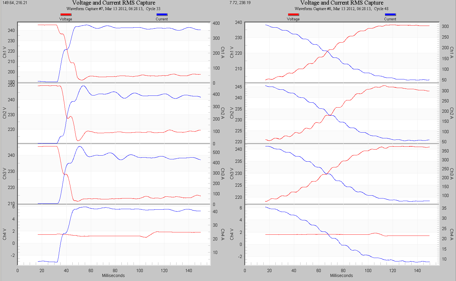
As shown in the previous whitepaper, and in Figure 9, a typical event lasts around 15 cycles, as determined by the timestamps of the two triggered waveforms (one for the event start, one for the end). So, our result from purely 1 minute stripchart data is very close, even better than the isolated calculation that required Significant Change data!

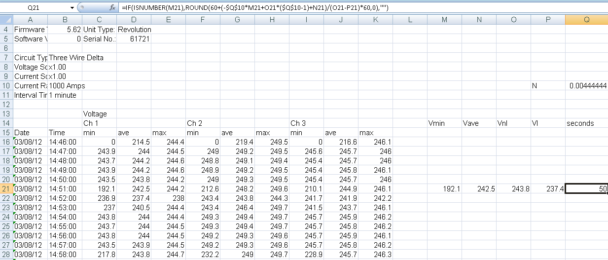
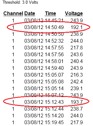
Now that we know the typical event duration, it’s actually possible to back-calculate the event timestamp within each interval. Rearranging the equation for N gives the formula for t. For data points within the linear region of Figure 6 (especially the 100 in the center), the calculation for the event timestamp is within a few seconds. Figure 10 shows a portion of the interval data with the “seconds” column added, showing the formula to compute the second value of the timestamp. As seen in Figure 11, the first two estimated timestamps are within one second of those reported in the Significant Change report.

Conclusion

A technique has been shown to extract cycle-level event duration purely from one minute stripchart data, with suitable clean data. The previous method relied fundamentally on the precise stripchart average in an interval, which is composed of the unloaded voltage, loaded voltage, and the very short sag voltage. Knowing the precise timestamp of the sag allows the sag duration to be computed, and the many cycles that go into the average calculation yields a very precise number. This new method relies on averaging again – this time, averaging the results of many events, eliminating the need to know the precise timestamp of any one of them. The result agrees even more closely with actual waveform data, and even allows for back-calculation of the actual timestamps.