Abstract
This white paper is an overview of Harmonic Vector Diagrams. The basics of 60 Hz phasors and harmonics are described, and steps for accessing harmonic vector diagrams in ProVision are reviewed. Almost no power circuit will be purely resistive. Large motors, transformers and similar devices can all create capacitive and inductive loads and contribute to harmonics. Reviewing vector diagrams can reveal a lot about how loads are impacting a distribution system.
Fundamental
The Fundamental is also known as the first harmonic. The most common example of the Fundamental Voltage Harmonic is a sine wave with an amplitude of 120V at a frequency of 60 Hz and a reference phase shift of 0 degrees. Ohm’s Law states that E=IR. A 120V supply with a purely resistive load, e.g. 1K ohm, would give a current sine wave with an amplitude of 0.120 Amps at 60 Hz with 0-degree phase shift.
In reality, almost no power circuit will be purely resistive. Large motors, transformers and similar devices can all create an inductive load. A capacitive load (mostly due to capacitors) is also part of the overall resistance known as impedance.
If an assumption is made that the standard of 0° is a purely resistive load, there will be no shift in phase from the voltage to the current waveforms. Thus, the two waveforms are said to be “in-phase”. That means that pure resistance only has an effect on the amplitude of the current wave and its phase is identical to the supplied voltage as shown in Figure 1.
When we begin to add other forms of impedance into the equation, the phase angle begins to change. One easy way to remember the impedance relationship is the phrase “ELI the ICE man”. The “E” represents the standard Electromotive Force or Voltage. The I is the standard variable for Current. The “L” in ELI stands for Inductive Load and “C” represents a capacitive load. Hence, ELI means that in an inductive load, Voltage leads Current. “ICE” means that in a capacitive load, Current leads voltage.
As seen in Figure 2, the current leads the voltage by 90°. The reason for the 90-degree shift is best understood if we think about a physical circuit. Consider a simple capacitor. When the capacitor is initially powered on, the voltage is zero. This is when the current is at its maximum flow rate. As the voltage cycle reaches its peak 90 degrees later, the rate of change is the slowest, so the current is a minimum. Because voltage is a sine wave, the current is also a sine wave.
The relationship between impedance and its individual components (resistance and inductive reactance) can be represented using a vector as shown in Figure 3. The amplitude of the resistance component is shown by a vector along the x-axis and the amplitude of the inductive reactance is shown by a vector along the y-axis. The amplitude of the impedance is shown by a vector that stretches from zero to a point that represents both the resistance value in the x-direction and the inductive reactance in the y-direction.
Each harmonic is a sine wave, like the 60Hz fundamental, just at a different frequency. The harmonic voltage and current sine waves at each harmonic frequency each has their phase angles, and the phase difference is computed just as it is for the fundamental. This gives a separate vector diagram for each harmonic. In most AC power systems, the even harmonics are mostly zero in amplitude due to cancellations in 3 phase systems, and the symmetries in most nonlinear load currents.
The odd harmonics are an integer multiplier of the fundamental. For example, if your fundamental harmonic is 60Hz, then the 5th Harmonic is 5 x 60 Hz, which would be 300 Hz. Also, bear in mind that a voltage harmonic at 300Hz only interacts with 300Hz current for the purpose of Phasor diagrams.
Accessing the Data
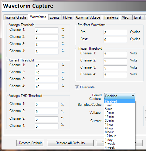
To access this data, you must first set up the unit to record waveforms, from which ProVision can compute and display harmonic vector diagrams. Since a standard initialization will only capture data during an out of spec event such as voltage sag or other waveform disturbance, it’s best to tell the monitor to record data at regular intervals. The periodic captures generate waveforms throughout the recording session, and “normal” waveforms are recorded.
To enable periodic waveform capture, select a time period under Period Capture. Figure 4 shows the Waveform Capture setup screen, with the period being set to 30 minutes. This period can range from 1 minute to 4 weeks, but the period should be so the waveform capture memory lasts roughly as long as the recording session. The number of waveforms, and time until memory is full, is shown in the Info section of the waveform setup screen. In this example, 318 waveforms may be captured, giving almost a week of recording time with 30-minute periodic captures.
Once initialized, make a recording using both Voltage and Current at the desired location. It’s then possible to download the data using ProVision Software, either by retrieving the recorder and manually downloading or by remote (Cell and Ethernet are both available). Once downloaded, select the file to be viewed from the Explorer Tab, usually in the “Recent Downloads” folder.
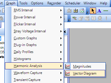
Once Downloaded, from the top toolbar, select “Graph”, then “Harmonic Analysis” and choose “Vector Diagram” as shown in Figure 5.
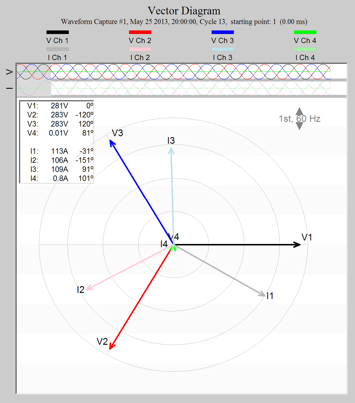
Once opened, the Vector Diagram Shows the Voltage and Current Vectors for each channel recorded. In the upper right-hand side of the page, the varying harmonic can be viewed by means of the arrow up or arrow down button. ProVision computes the vectors for each harmonic for the waveform cycle covered by the grey rectangle at the top of the graph – move this rectangle through the waveform capture to select a representative cycle. If the capture was triggered by a voltage sag or other disturbance, move this to a “normal” cycle in the capture.
Looking at the vector graphs shows the amplitude of the harmonic, and makes it possible to determine whether the phase angle is capacitive or inductive. It is also possible to view which harmonic is largest so appropriate actions may be taken. Figure 6 represents a standard 3 phase source, with each phase voltage separated by 120° and a current which leads its Voltage phase by 31°. This result is typical of a delta circuit with an inductive load.
In order to view the Magnitude of each harmonic simultaneously, click on the Harmonics graph button in the Real Time Waveforms Toolbar. In the example shown in Figure 7 most of the data is well below the magnitude of the Fundamental Harmonic.
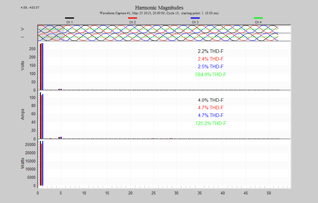
Remove the First Harmonic data from the graph with a right mouse click anywhere in the graph area and uncheck the “Show Fundamental” option.
Determination of Power Flow
Each current probe built by Power Monitors Inc has a power flow indicator, usually an embossed arrow at the joint location. In normal operation, the phase angle between the voltage and current should be between 0° and +/- 90°. If the phase angle between the voltage and current is more than 90 degrees apart, this usually means that the current probe used with a power/harmonic meter or analyzer is placed in opposite direction of the assumed power flow. The arrow should be pointing in the direction from the source to the load, which is the normal direction of power flow. When the phase angle of the harmonic voltage and current is between 90 degrees and 270 degrees (270 is also referred to as -90 degrees) on a properly installed CT, then it is assumed that this harmonic power flow is in the opposite direction of the fundamental power flow, or from load to source.
Conclusion
An understanding of the basics of 60 Hz phasors and harmonics and proper assessment of the vector diagrams generated by periodic waveforms make it possible to get a good idea about how capacitive and inductive loads are impacting a distribution system. ProVision can graph the vector diagram for the 60Hz fundamental, and any harmonic, as computed from the recorded waveform capture data. The fundamental phasors show the bulk 60Hz voltage, current, and power relationships while the harmonic phasors reveal phase shift information for more specialized troubleshooting.
