Abstract

Many AMR (automatic meter reading) systems rely on PLC (power line communication) signals for data transfer. These signals travel on the 60Hz distribution network and can be affected by power line noise and attenuation. Troubleshooting PLC-based AMR systems requires measuring signal and noise levels at comparable levels and bandwidths to the PLC system itself, directly on the 60Hz system. The Revolution can measure the larger outbound data signal with interharmonics. Further, a method is shown to capture the very small inbound signal with a detailed waveform capture analysis. These measurements can aid in finding interfering noise sources or null spots that attenuate PLC signals.

TS2

One popular AMI system is TS2 (patents 7,102,490 and 7,236,765). This bidirectional data system uses a clever method to trade off speed for low power and reliability. A fundamental communications theory result is Shannon’s law, which relates the channel capacity C (bits per second) to the system bandwidth B (Hertz), and the signal and noise powers (S, N, both in Watts). For a given channel, to increase the data rate C (assuming the channel was already at maximum capacity), you must either increase the bandwidth, increase the signal power level, or somehow reduce received noise. Conversely, if a very low power or narrow bandwidth is needed, the data rate must be reduced.

The TS2 system carries this principle to an extreme by taking advantage of the low data rate required for AMR. Reading a revenue meter daily is usually sufficient, and this involves just a very few bytes of data. By spreading the small data packet over a long period, the required signal level and bandwidth can be made very small, allowing the signal to coexist with the 60Hz power line without interference, and also allowing many parallel channels to exist (one for each revenue meter). The inbound (meter -> substation) signal data rate is around 20 minutes per bit, and results in a meter reading roughly every 20 hours. This slow data rate allows for a very low power transmitter at each revenue meter, and results in a very narrow bandwidth per channel – just 0.004Hz wide! The TS2 system packs 9000 separate channels between the 16th and 17th harmonic (960Hz – 1020Hz), and the 4mHz x 9000 channels fits in a 36Hz band for the entire inbound system. The transmit power from each revenue meter is extremely small at under 1 Watt, and the voltage signal at the revenue meter is just a few millivolts. The very slow rate of 20 minutes per data bit allows for very heavy synchronous averaging on the substation receiver side; this averaging technique allows the very small signal to be separate from the non-synchronous noise, in keeping with the Shannon equation.

The outbound (substation -> revenue meter) signal characteristics are not as extreme. Two carriers are used, one at 555Hz, and one at 585Hz, to indicate a binary zero or one. Since only one transmitter is used to broadcast over the entire distribution circuit, only one outbound channel is needed. Also, the outbound power level is much higher since the equipment can be installed in the substation vs. under the meter glass. The two signaling frequencies (555 and 585Hz) are located between the 9th and 10th harmonic. The frequencies and timescales involved are in the audio range, and it’s actually possible to hear the two tones at the substation transmitter (due to slight vibrations in the wire from the magnetic force generated from the pulse current). The tones can also be extracted via signal analysis from the powerline itself. In this recording, 60Hz and all harmonics have been digitally removed, leaving just the two PLC tones at 555 and 585Hz, alternating to transmit zeros and ones.

These TS2 characteristics are designed for reliable PLC communications, and are well designed for slow PLC signaling without interfering with or being interfered by typical 60Hz power line noise. However, the properties that let them “hide” in the 60Hz systems present a challenge in capturing TS2 signals with a conventional power quality meter. The signals are well below 1V RMS, are nestled completely between pairs of harmonics, and typically require many seconds or minutes of averaging to be reliably detected by standard TS2 receiver with special narrowband filtering. To troubleshoot a TS2 communications issue, a method for measuring noise and signal levels is given for the Revolution.

The outbound signal is easier to capture. The two signaling frequencies, 555 and 585Hz, are conveniently located on two standard interharmonics between the 9th and 10th harmonic. Although just measuring these two interharmonics is enough to measure the outbound signal level, the region around these frequencies is important to capture for assessing noise levels.

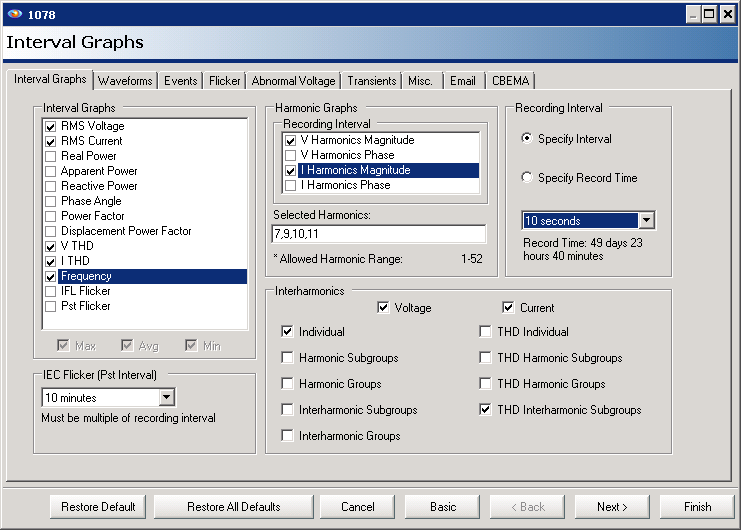
The recommended setup is shown in Figure 1. Harmonics 7, 9, 10, and 11 are chosen for recording, and by checking “Individual” in the interharmonic section, all interharmonics between those harmonics are also recorded, including 555 and 585Hz. The interharmonic subgroup THD is enabled, which is useful in quantifying the amount of total interharmonic distortion vs. “regular” harmonic distortion. A 10 second stripchart interval is shown, but a 1 minute interval could be used for a longer recording time, or if more stripchart data were required for other PQ issues.

For this whitepaper, a Revolution was used at a residential location covered by a TS2 system. The channel 1 voltage input was connected across the 240V service, and the other channels unused – this gives the maximum voltage resolution for PLC analysis. The injected and received signals at the revenue meter do not involve the neutral, and the Revolution should be connected to match this.

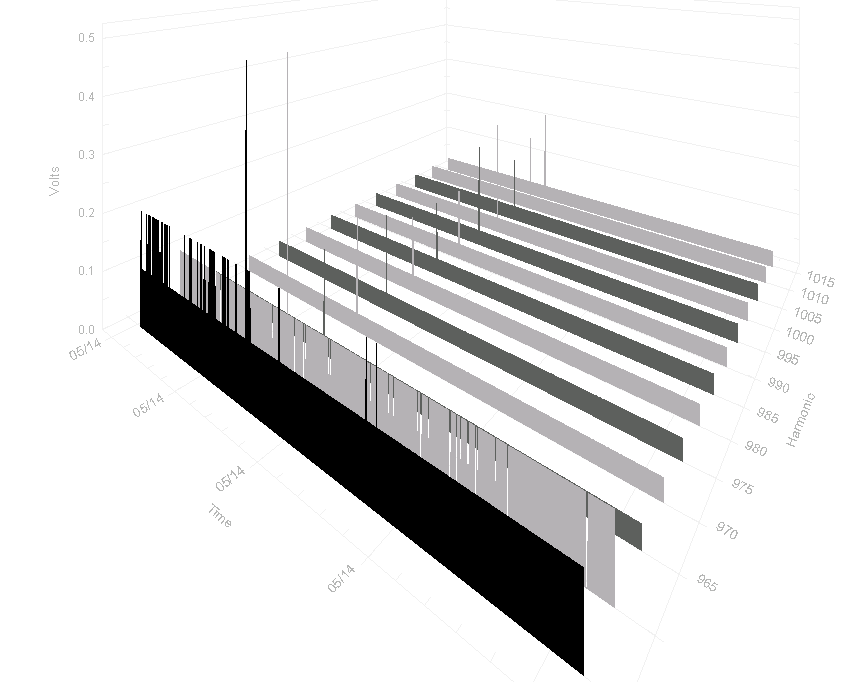
The area around the outbound signal is shown in the 3D ProVision harmonic plot (Figure 2). The 555 and 585Hz interharmonics are in red, and the others in grey. At around 2V RMS, the 9th harmonic is small, but still much larger than the PLC signals. The two signaling frequencies are well under 1V RMS, but still noticeably higher than the surrounding interharmonics. This 3D view is good for seeing at a glance the relative level of the 555 and 585Hz carriers compared to the adjacent interharmonics. In a noisy environment, the surrounding interharmonics (e.g. 550, 560, etc.) will be large compared to the signals, and the overall levels will vary much more over time. Usually noise sources such as arcing, VFDs, etc. will come and go intermittently, and this should be readily visible in the 3D graph as a wide-band change in level.

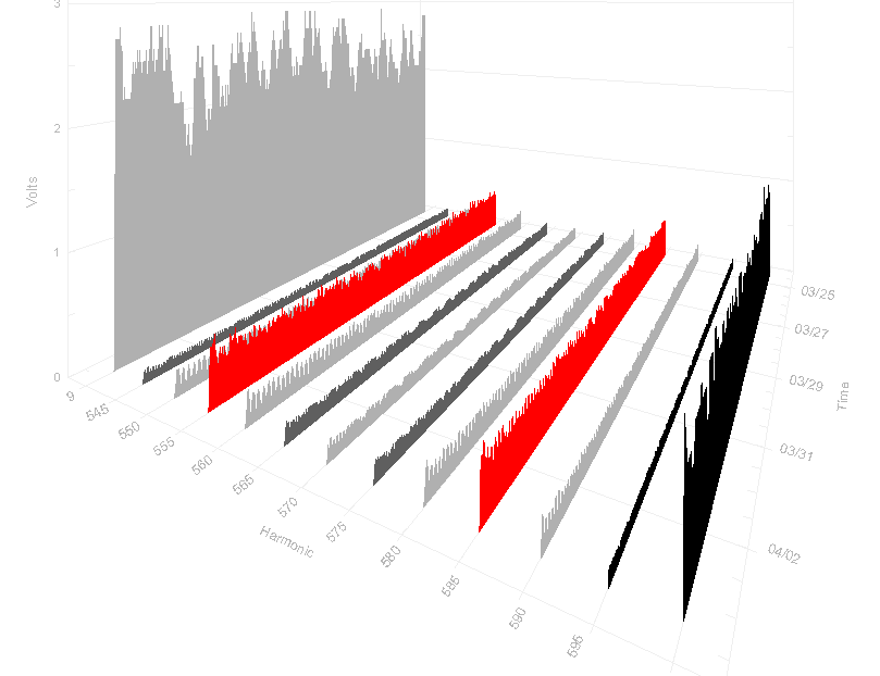
In this recording the 1 minute stripchart interval is long enough that the average outbound signal was constant for each interval, and the small variations seen in the graph are due to actual system impedance changes. Large system impedance changes (e.g. due to a cap bank switching in or out) can cause signal attenuation, sometimes enough to prevent proper signal reception. The 3D graph would show this as a large change in the red trace amplitudes at certain times. The noise may or may not change at the same time, depending on the relative location of the noise source with the system impedance change.

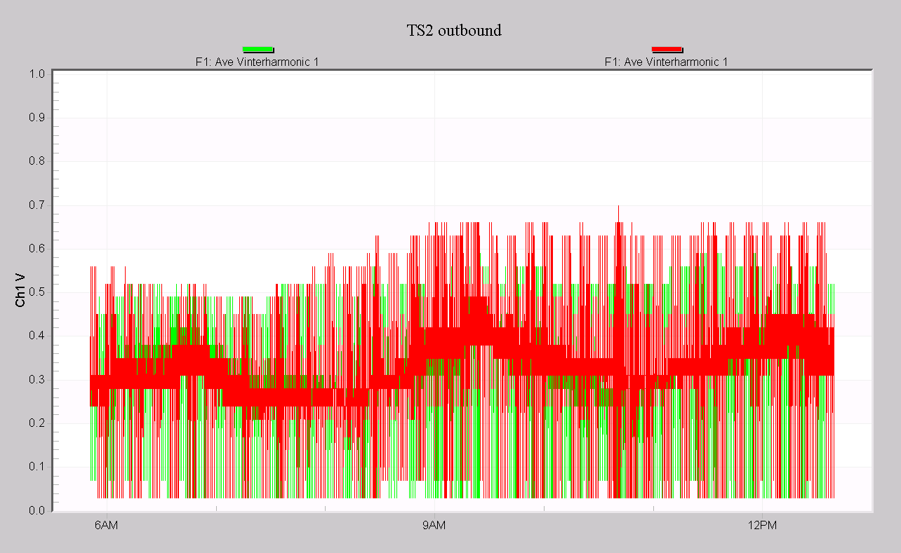
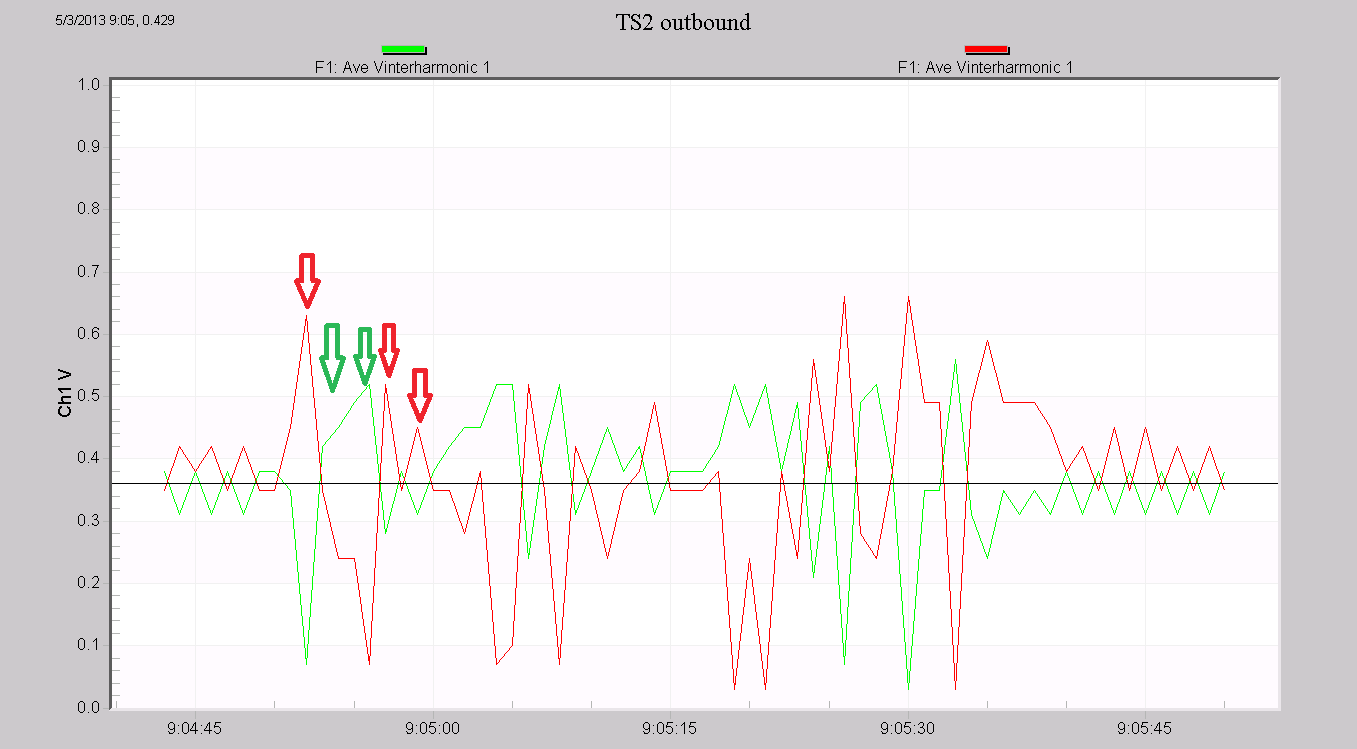
The individual interharmonic stripcharts can be used for a more detailed view. In Figure 3, a custom graph was created showing the 555 and 585Hz carriers, this time with a 1 second interval (different recording, but same location as Figure 2). With this resolution it’s possible to see the individual transmit periods for data blocks. Zooming in even further, Figure 4 shows individual bits, or groups of bits, the first few indicated by arrows. A horizontal reference line has been drawn around 0.36V, which appears to be the baseline value that separates a “signal” from “no signal” level.

The 3D graph is best used for noise or interference problems. “Broadband” noise caused by non-synchronous loads (arcing, VFDs, inverters from photovoltaic or other generation, etc.) will span many interharmonics, and a view that shows them all is useful. The 2D stripchart plots are most useful for looking at system impedance changes that attenuate the signals – in this case, adjacent frequencies aren’t as important, and the actual signal levels are, which are easier to see on the 2D graph.

Capturing the inbound signal from the revenue meter is much more difficult. For this direction, the substation receiver diagnostic output is often helpful, including received signal strength vs. time for a particular channel. This isn’t available anywhere but the substation though. It is possible to measure this with a Revolution with a more advanced analysis.

The inbound voltage signal at the revenue meter is often just a few millivolts, tiny compared to the 240V 60Hz voltage. In addition, the specific meter signal is surrounded by 9000 other signals in the 36Hz wide TS2 band. Resolving one particular meter requires a lot of averaging – the substation receiver is averaging for 20 minutes to detect one bit of information. Although 20 minutes isn’t needed to just measure the signal at the meter, more data than the 12 cycle IEC interharmonic window is needed. Per the IEC 61000-4-7 standard, the Revolution uses a 12 cycle capture window, giving a 5 Hz resolution per interharmonic. This is not sufficient for isolating the inbound signal; to do this, the data must be captured manually and analyzed.

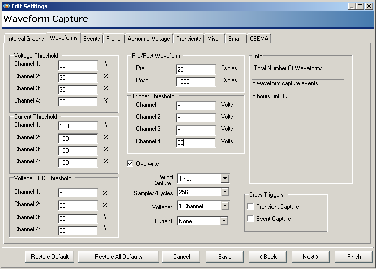
The raw waveforms are captured with the Revolution, then analyzed outside of ProVision to extract the PLC signal. Figure 5 shows waveform capture setup for this. An extreme waveform length of 1020 cycles is used – over 16 seconds per capture – for a good averaging length. To maximize the waveforms, only one channel of voltage is used, connected across the 240V service. Periodic capture is used to capture a “normal” 10 second stretch, rather than analyzing a triggered waveform from a PQ event. The trigger values have been set to high thresholds to prevent any non-periodic captures. Although usable data can be gathered with a little as 3 or 4 seconds, the longer the better.

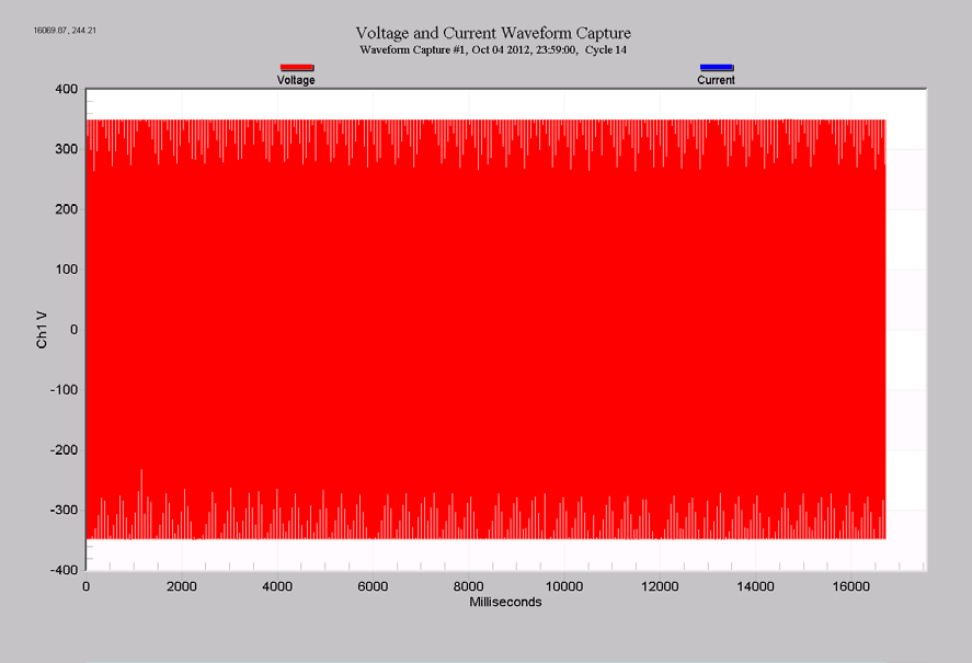
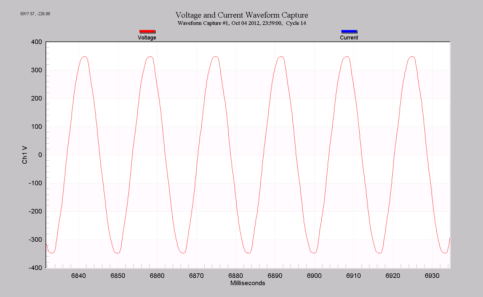
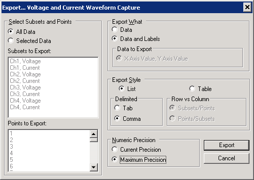
A raw waveform capture is shown in Figure 6. All 16 seconds are shown, and at this zoom level the individual cycles aren’t visible. Zooming into a random section (Figure 7) shows a normal-looking 240V RMS sine wave. The interharmonics between the 16th and 17th harmonic were recorded (Figure 8), but the results are essentially at the noise floor, hovering around 0.03V RMS. The real inbound signal is ten times smaller, and we need to dig deeper. To go further, the data must be exported from ProVision and imported into a signal processing tool such as Matlab. From within the waveform capture graph, right-click on the graph and choose “Export Dialog.” Then, choose Text/Data, and File for the destination. A details form will appear; Figure 9 shows the best settings for easy importing into Matlab.

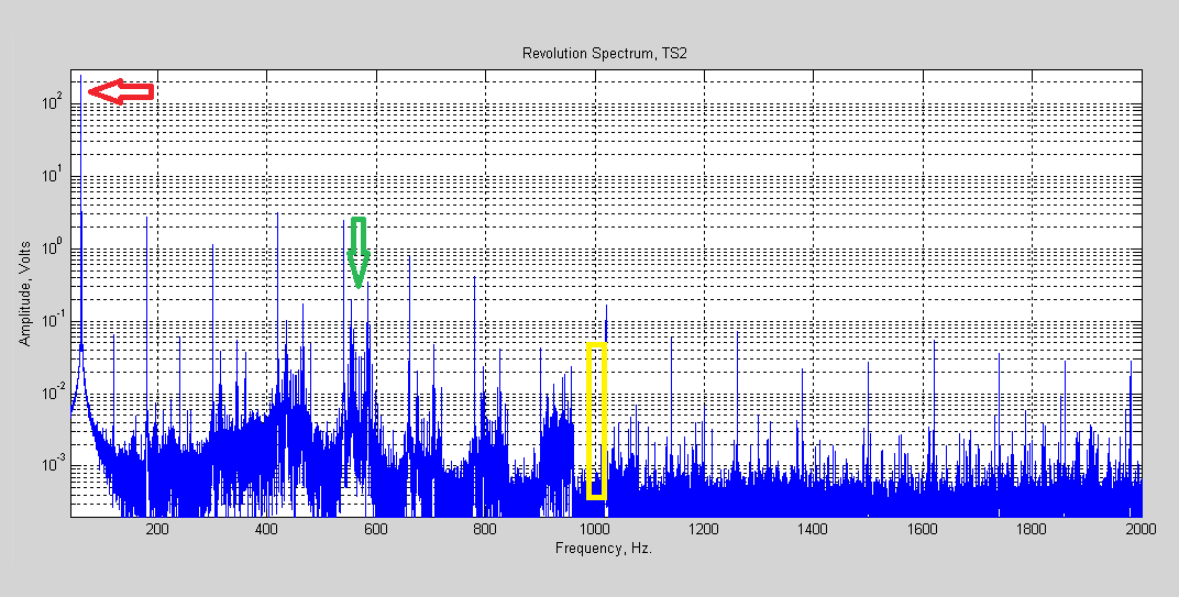
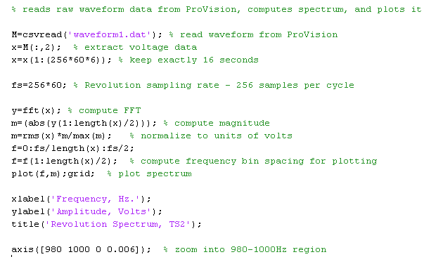
The file can be read directly into Matlab with the csvread command. The entire 16 second capture, over 245,000 points, was analyzed with the FFT command. With this many samples, the frequency resolution is 60/(16*60) = 0.065Hz. This isn’t enough to resolve a single 0.004Hz channel, but is enough to examine the band in some detail. The resulting spectrum is shown in Figure 10, with a logarithmic y-axis. Of course the largest signal is the 240V 60Hz component, shown with the red arrow. The 60Hz harmonics are thin blue lines, the odd harmonics over 1V up until the 9th, and the even ones down below 0.6V. The 555 and 585Hz outbound carriers are visible, as shown by the green arrow (note that they’re not much bigger than the even harmonics). The entire 36 Hz inbound band is highlighted in yellow, and at this zoom level nothing’s yet visible.

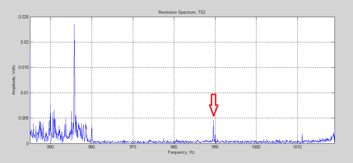
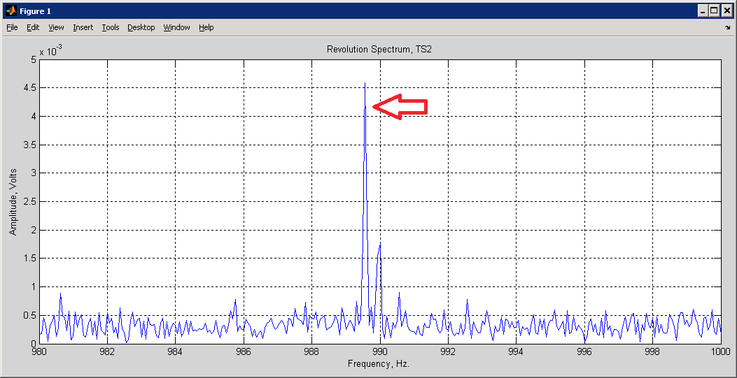
Zooming in further (Figure 11), we can finally see some inbound data. The entire 9000 channel band resides between 970 and 1006Hz; anything outside of that is noise. The only in-band signal here is near the red arrow. Zoom in yet further (Figure 12) and the actual meter in this location is seen. This meter happens to be channel 15743 in the TS2 system, which corresponds to a frequency of roughly 989.9Hz. Figure 12 shows that the main peak is very close to this value. The signal level is around 4.5mV, or 0.0045V RMS, roughly 50,000 times smaller than the 240V AC line, almost 800,000 times smaller than the max input to the Revolution (designed for ± 5000V transients). The Matlab listing for this analysis is shown in Figure 13.

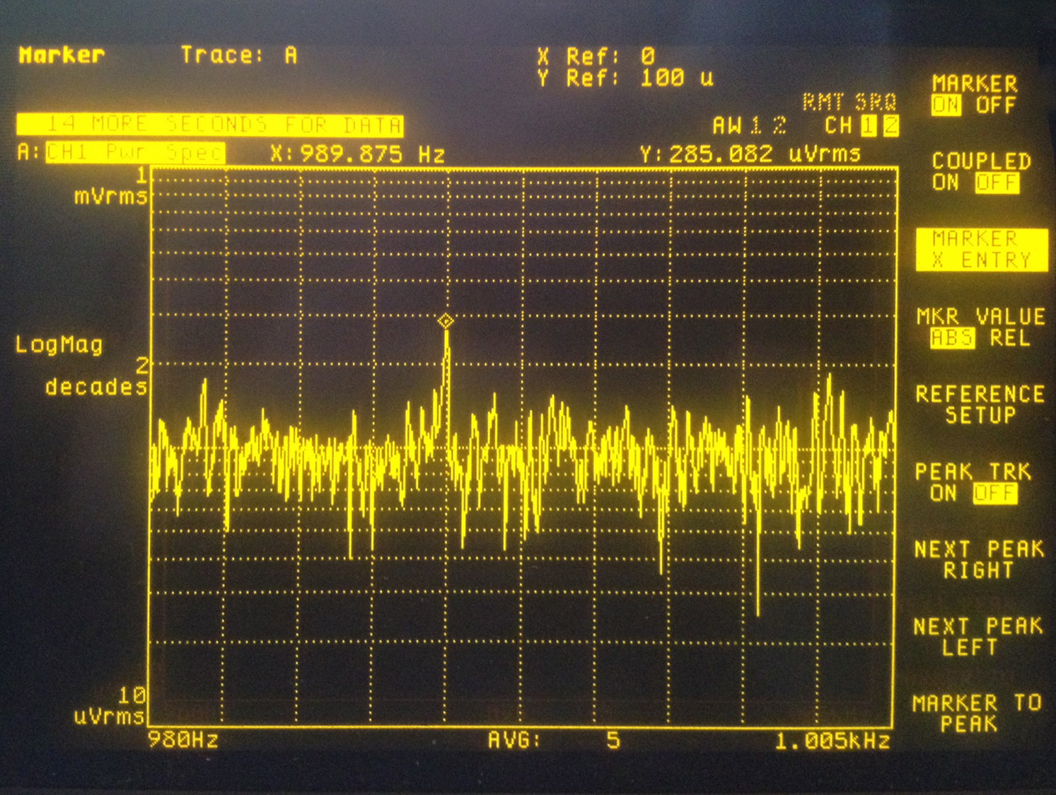
This result was checked with a Hewlett Packard 35670A audio-band spectrum analyzer, connected directly (carefully!) to the 240V line. Figure 14 is a screenshot of the spectrum zoomed into the inbound band. The peak at 989.875 is the TS2 signal, here at a level of 2.8mV RMS, a bit less than it was during the Revolution recording (a 10X probe was used, making the on-screen measurement off by a factor of 10). The spectrum analyzer required over 70 seconds of averaging to achieve this resolution.

For troubleshooting the inbound connection, the recording at the revenue meter can be used to confirm that the meter is transmitting and is at the expected frequency. Since the receiver is at the substation, further measurements would start at that point using the substation receiver tools, and proceed to possible interference sources along the circuit back to the meter.

The inbound band is between the 16th and 17th harmonic, so recording all interharmonics between them can be useful for measuring interference. Although the resolution is only 5Hz, this bandwidth is adequate for looking at interference, even if over 1200 channels are contained in it.

Conclusion

Methods have been shown to measure TS2 AMI signals, both outbound and inbound. In general, the 3D harmonic/interharmonic plots are most useful for measuring noise sources, since that view emphasizes an all-band view vs. high resolution in amplitude or time. The 2D stripchart plots are best for examining transmitted signal levels, attenuation, or changes in system impedance, since these are primarily needed at the actual signaling frequency, and a good amplitude resolution view is needed.

The outbound signal is easily measured with just interharmonic recording, since the carriers are at exact interharmonic frequencies, the data rate makes them relatively wide band, and the signal levels are relatively large. Since spectral plots aren’t available at each revenue meter, a portable PQ analyzer that can measure the received substation signal is very helpful.

The inbound signal is much more difficult to capture, and requires many seconds of raw waveform capture for adequate amplitude and time resolution. Despite this, the Revolution hardware is capable of revealing signals at the millivolt level with some outside help from Matlab. For everyday inbound troubleshooting, this shouldn’t be required, and regular interharmonic analysis from the 16th to the 17th harmonic can be enough to track down noise sources, and the substation receiver spectral plots can be used for system impedance and attenuation issues (which isn’t available at the revenue meter receiver).