Abstract

Traditional harmonic analysis in electrical systems has revolved around looking at the spectral content on, well, the magnitudes of harmonic frequency components. The IEEE 519 specification provides guidelines for measuring and quantifying the effects of these harmonics. However, voltage or current components can be present between these harmonic frequencies and can present their own special symptoms and challenges in mitigation. These components are called interharmonics and are measured using 5Hz frequency intervals. The reader is encouraged to consult IEC 61000-4-7 for the full definitions and recommendations regarding measuring interharmonic content.

This whitepaper will be discussing the specifics of performing an interharmonic analysis using the Python programming language.

Prerequisites

Of primary importance is the inclusion of an embedded set of binaries in this library. libnative.dll, libnative64.dll and the corresponding FreeBSD and Linux .so files are embedded in a Python script within this library. On *NIX systems, the system library paths (/usr/lib/ and /usr/local/lib/) directories are searched first. If they do not exist then “.” is searched. If the requisite binaries do not exist in any of those locations, then the ml_canvass library will automatically extract the needed binaries in the working directory.

For Windows systems this is not the case. Since there are multiple Python distributions and Windows versions, and ActiveDirectory and permissions issues, the ml_canvass library never attempts to look in a “system path” for the included libraries. It always looks in the current working directory (“.”) and extracts the corresponding libraries (if needed) based on register bit-width of the executing version of Python.

Additionally, the ml_canvass library requires that the following Python packages be installed as well:

• numpy
• matplotlib

NOTE: When determining the register bit-width of windows machine, the following code is executed:

from ctypes import *
reg_width = sizeof(POINTER(c_char))*8

Getting Started

With the prerequisites out of the way, the reader can now download and install the ml_canvass library. (See the links section at the end of this paper for the download.)

Once downloaded, the user should use the pip command to install the library. It should look something like:

pip3 install ml_canvass-1.2.3-py3-none-any.whl

Note that the filename may change. Use the filename from the download section at the bottom of this page.

To test that the installation was successful, launch the interactive Python runtime and execute the following import statement:

from ml_canvass.nsf_recording import nsf_recording

If the command returns without error, then the library has been successfully installed. If it has not, then the user is urged to follow the resulting stack trace and work backward through the errors to resolve the issue.

Analyzing a Waveform Capture for Interharmonics

As mentioned in IEC 61000-4-7, waveform capture recommendations are for a minimum of 12 cycles:

where is the bin width in Hertz of the resulting DFT, is the sampling frequency and is the number of samples.

PMI recorders sample waveforms at 256 samples per cycle (not including transient capture which is 1 MHz sampling rate). Consequently and appear in the equation above. A simple factoring shows that the 256 cancels leaving.

(See White Paper #73, Harmonics from Periodic Waveform Capture for more information on configuring a PMI PQ recording to record periodic or triggered waveform captures that span 12 cycles.)

The reader should take note that even if the recording in question does not contain a full 12 cycles (or even contains more than 12 cycles) per waveform capture, the ml_canvass interharmonics module can still be used. The library will either zero-pad (which will lead to attenuation in the magnitudes of the individual frequencies) short samples or take the first 12 sub-samples for long samples and perform the FFT on those.

The module in question is the ml_canvass.interharm module. It can be imported with the following statement:

from ml_canvass import interharm as ih

The “as ih” clause is an aliasing clause that allows the programmer to reference the interharm module without having to type “interharm” every time, but just “ih” instead.

There are currently (as of the time of this writing) two functions that are exposed as part of the interharm module:

• interharm_mags(points, samples_per_cycle)
• harmonic_group_mags(iharm_mags)

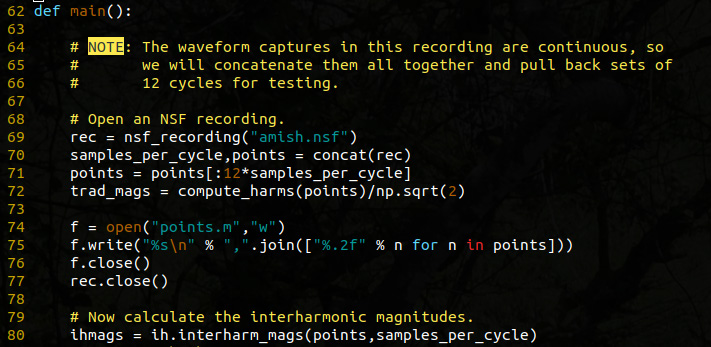
The first function returns an ndarray (NumPy array) of instantaneous magnitudes for all component frequencies from DC to. (The output is only one half of the length of the sample since the inputs are real-valued inputs for the DFT.) Figure 1 shows a source code example of how to invoke that function and Figure 2 shows the resulting graph.

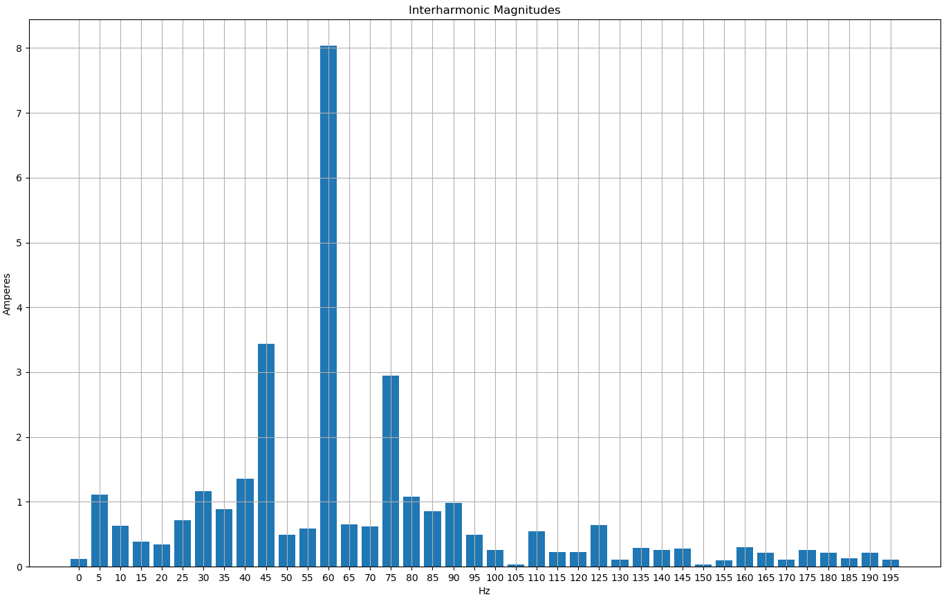
In Figure 2, take special note of the dominant interharmonic frequencies: 45Hz and 75Hz. Compared to the integer multiple harmonics of 120Hz, 180Hz, 240Hz, etc. interharmonic magnitudes are significantly stronger.

Code Dissection

The source code snippet from Figure 1 shows the application entry point main() and a source code note about the recording that was produced for testing. The THD (as specified by IEEE 519) for the waveform captures was at ~11% for a sustained period, resulting in a series of waveform capture records that were sequential. The waveform capture records themselves were only 9 cycles in length, but because they were contiguous in time, they were concatenated together for the purposes of IEC 61000-4-7 interharmonic analysis. The source code for concatenating the waveform captures can be found in the included demo source code in interharm_demo.py starting on line 37.

Lines 74 through 76 were retained in the source code, but are not strictly necessary. For users who prefer MATLAB or Octave (the GNU open source clone of MATLAB) these three lines will generate a MATLAB file called points.m that contains a single array of all of the concatenated waveform values. That array can then be loaded into MATLAB or Octave with the load command and subsequently analyzed using the different toolkits that the user may have installed. (It is perfectly acceptable to comment out or delete these three lines if the user does not intend to use MATLAB.)

Line 77 closes the recording since it is no longer needed and, finally, line 80 is the line wherein the interharmonic magnitudes are calculated. On this line, the raw time-domain waveform sample (points) is passed as the first parameter while the number of samples per cycle (samples_per_cycle, which was retrieved from the recording with a value of 256) was passed as the second parameter. As mentioned previously, the return value from this function is an ndarray of instantaneous magnitudes.

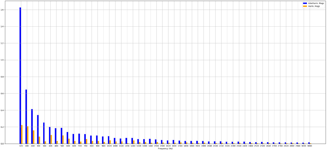
The blue bars in Figure 4 represent the harmonic group magnitudes while the orange bars show the IEEE 519 harmonic magnitudes. As is evident in the graph, the harmonic group magnitudes are significantly larger than their counterparts. This will result in a harmonic group THD that is many times larger than the IEEE 519 THD. Take special note of the strong even harmonic group magnitudes (at 120Hz, 240Hz, etc.), especially as compared to the IEEE magnitudes. A quick glance at “traditional” harmonic magnitude reports may not yield any big “surprises”, but the harmonic groups show a significant amount of energy in the intermediate frequencies. In this particular data set, the strong interharmonic content at 45 and 75 Hz indicate a possible light flicker power quality problem.

Line 81 is a call to the second interharm module function: harmonic_group_mags. This function takes the frequency domain values calculated earlier with interharm_mags and returns a new ndarray with the interharmonic magnitudes for each of the harmonic frequencies (60Hz, 120Hz, 180Hz, etc.) through the 52nd harmonic.

The harmonic group magnitudes are calculated according to the IEC 61000-4-7 specification as set forth in section 5.5.1 Grouping and Smoothing. As per the specification for a 60 Hz system, group magnitudes are calculated as follows:

Following the code listing in Figure 3, starting on line 85 an x-axis array is being generated based on the length of the interharmonic magnitudes calculated above on line 80.

Lines 87 and 88 are used to truncate the interharmonic magnitude array and the x-axis array to the 200Hz entry to prevent crowding in the resulting graph. This isn’t necessary, but does make for a better presentation. Of course, it does also truncate data, so care must be taken to remember that what’s being displayed is literally not the “whole picture.”

Finally, lines 90 through 99 are used to plot the interharmonic spectrum as a bar graph. Take special note of line 92. The second parameter to the bar() function for matplotlib is:

ihmags/np.sqrt(2)

This is an in-place scalar division on a vector. It’s converting the instantaneous magnitudes to RMS magnitudes for plotting.

Lines 101 through 117 are used to generate a graph of interharmonic magnitudes vs “traditional” IEEE 519 harmonic magnitudes. The IEEE 519 magnitudes were calculated on line 72 and are plotted alongside the IEC 61000-4-7 interharmonic magnitudes as seen in Figure 4.

Conclusion

Interharmonic analysis can be an important tool when diagnosing power quality problems, especially with non-traditional loads. This whitepaper has demonstrated how that analysis can be done with relative ease using PMI’s PQ recorders and the Python programming language.

References and Downloads

• ml_canvass Library Installer for Python
• Harmonics from Periodic Waveform Capture
• Net Metering in ProVision