Abstract

In a normal distribution network, the fundamental frequency is that of the voltage driving source, nominally 60Hz. Steady state deviations from the ideal 60 Hz sine wave shape are “periodic,” which allows for a useful method of analysis. A periodically distorted waveform may be decomposed into a combination of sine waves with multiples of the powerline frequency; these are known as harmonics. The harmonic number indicates the integer frequency multiple e.g. the 1st harmonic (the fundamental) is 60 Hz, the 2nd is 60 x 2 = 120 Hz, 3rd is 60 x 3 = 180 Hz, etc. This decomposition into harmonics is only valid if the waveform distortion is the same every cycle, thus harmonics are a steady state PQ problem.

Harmonic Results From “Non-Linear” Loads in an Electrical System

Any waveform that deviates from an ideal sine wave has harmonic components. Most nonlinear loads draw harmonic currents and therefore produce harmonic voltage distortion by producing non sinusoidal voltage drops across system wiring and transformers.

These are specified by their harmonic number or multiple of the fundamental frequency. For example, with 60Hz fun damental frequency the third harmonic is 180Hz. In this example, for every cycle of the fundamental frequency, there are three cycles of the harmonic frequency (180 Hz). Any complex, periodic waveform can be uniquely broken down in terms of harmonics, making harmonic analysis a useful way of analyzing nonlinear distortion.

This paper describes how harmonics are calculated from time series voltage and current waveform datasets.

The Discrete Fourier Transform – DFT

Fourier transforms are used to decompose times series data into individual constituent frequency components. The Discrete Fourier Transform (DFT) is defined as shown in Formula 1.

The output of the DFT has the same number of points as the input. Frequency resolution of the Fourier transform output depends on the number of cycles (the total number of fundamental periods passed to the DFT).

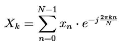
Here x[n] represents the nth time series sample in one period of a sampled waveform, which is N total samples long. X[k] is the kth output of the DFT, and represents the complex output. The complex exponential expression based on e can be interpreted as a combination of a cosine and sine function.

The DFT can be expanded using the Euler identity as shown in Formula 2 where k is the harmonic number (or DFT bin number), n is the time domain sample number, N is the number of points in the DFT input and Xn is the nth time domain sample. This more clearly shows the connection to sinusoidal functions.

Each output bin of the DFT calculation is always a complex number. K0 is the DC component and K1 is the
Fundamental. K2 will be the second harmonic, K3 the third and so forth.

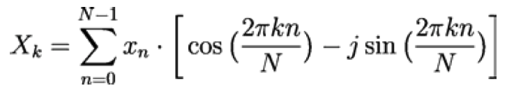
Formula 2. Expanded DFT Equation Using Euler Identity

For example, to find the third harmonic with 1 cycle of data and 256 samples per cycle, k is 3, N is 256 you get formula 2. The third bin is the third harmonic for a single cycle DFT.

IEC 61000 4 7 defines a standard method of measuring the frequency spectrum of the voltage and current signals; the standard defines the measurement window width for 60Hz systems to be 12 cycles. This 12 cycle length results in 5 Hz frequency bins. The IEEE Std 519 2022 also specifies the 12 cycle sampling and defines the harmonic component magnitude to be the center frequency combined with the two adjacent 5Hz bin values. The three values are combined into a single RMS value. This combination of three 5Hz values is also defined as the harmonic subgroup.

With multiple cycles (and by definition more time domain samples) you get more data points and more granularity of the output. The bin width is the sampling frequency divided by the number of sampled points as in formula 3.

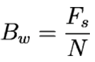
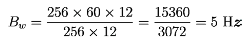
For example, if you have 12 cycles, 256 samples per cycle and 60 cycles per second, then the Bin width is shown in formula 5 which gives 5Hz bands.

For example, to find the third harmonic with 12 cycles of data with 256 samples per cycle, k is 3, N is 12 x 256 = 3072. The third harmonic is at 3_x60 = 180H_z . To find the bin width,
divide the frequency by the bin width 180|5 = 36.

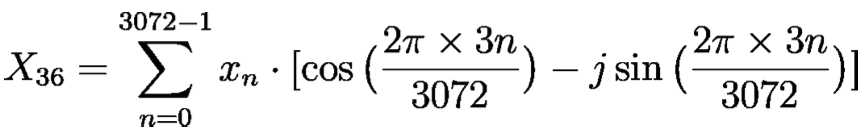
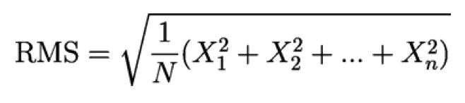
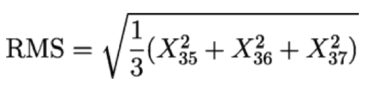
The third harmonic is at the center of the 36th bin. According to the IEEE Std 519 2022 is is to be combined with the three bins 35 37 as an RMS value. RMS values are the square root of the arithmetic mean of the squares of the value.

In this example:

Harmonic Magnitude and Phase Angle

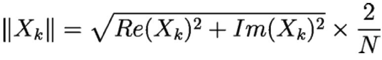
Given the complex harmonic value from Formula 2 we can find the harmonic magnitude and phase angle. The harmonic magnitude is found by taking the square root of the sum of the squares of the real and imaginary parts of the complex value. The kth harmonic magnitude is given by Formula 4. The 2/N is a normalization constant for the real valued inputs to the DFT.

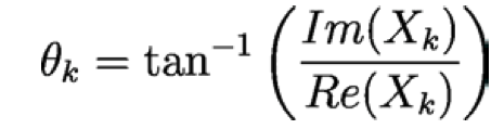
The harmonic phase angle is found by taking the arc tangent of the imaginary part divided by the real part of the complex value. The kth harmonic phase angle is shown in Formula 5. This phase angle is in radians.

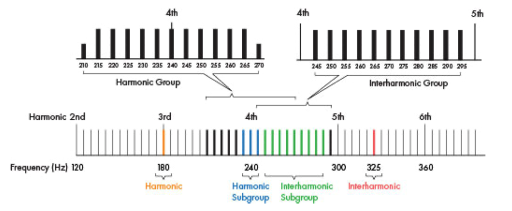
Interharmonics and Harmonic Groups

IEC 61000 4 7 defines the raw interharmonics as the frequency components every 5Hz, excepting the integer multiples of 60Hz (which are harmonics, not interharmonics).

Now that we have computed the harmonics in 5Hz bins using a 12 cycle sampling window we can use these to find the interharmonics, harmonic groups, and interharmonic groups.

A harmonic group is a combination of a specific harmonic and the surrounding interharmonics. There is a harmonic group for each harmonic. For a harmonic group the six preceding and six following interharmonics are combined with the harmonic itself with an RMS summation.

Harmonic subgroups are formed by taking the RMS sum of a harmonic and the adjacent interharmonics.

Interharmonic subgroups are defined as the RMS sum of the 9 interharmonics between two specific harmonics, not including the two interharmonics immediately adjacent to the harmonics.

See PMI’s whitepaper titled Defining Interharmonics for more detail on interharmonics and groupings.

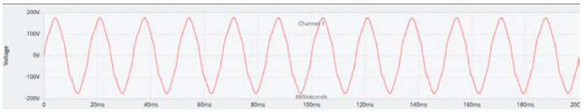
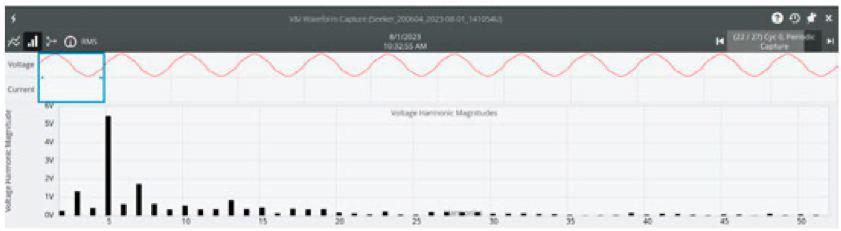
In PQ Canvass, users can quickly and easily perform harmonic analysis by looking at waveform capture records. Figure 1 shows a waveform capture in the time domain. Figure 2 shows the same waveform with the voltage magnitudes with the fundamental harmonic turned off.

Conclusion

Harmonics and interharmonics can be computed by used a DFT on the raw time series waveform data. Samplings of 12 cycles provides the needed granularity for computing interharmonics. This frequency decomposition is a powerful way to analyze waveform distortion.