Introduction

Harmonic Analysis is a fundamental part of any power quality investigation. A good amount of information can be gained about a power signal by looking in the frequency domain at what happens to various multiples of the 60 Hz line frequency. The core concept behind how any power quality recorders calculates this harmonic information is the Fast Fourier Transform or FFT. This concept is not limited to power quality analysis however. It is regularly used in any industry related to signal processing, including communications, image compression, physics measurements, audio engineering, radar, mechanical vibration, and many more. The goal of this white paper is to give some intuition behind this FFT concept so that it can be less of a magic black box and more of a reasonable and useful tool.

The Fourier Transform

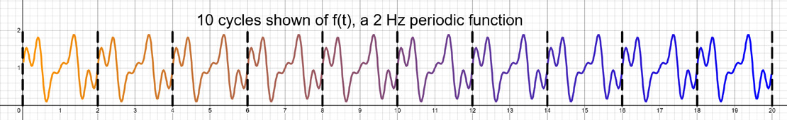
Take some arbitrary function ƒ(t) defined over some time interval, [a,b]. As an example, I have chosen some continuous periodic function with period 2 seconds that is defined from t = 0 to t = 20. This function is shown in Figure 1.

Now imagine evenly wrapping this function around the unit circle in a clockwise manner at some frequency w wraps per second, where each point (t,ƒ(t)) is mapped into polar coordinates with the radius given by r = ƒ(t) and the angle given by θ = -2πwt radians. The angle θ = 0 is on the positive horizontal axis. This can be neatly encoded in the complex plane by ƒ(t)· e^(-2πiwt). Several of these polar coordinate mappings are shown in Figures 2-6.

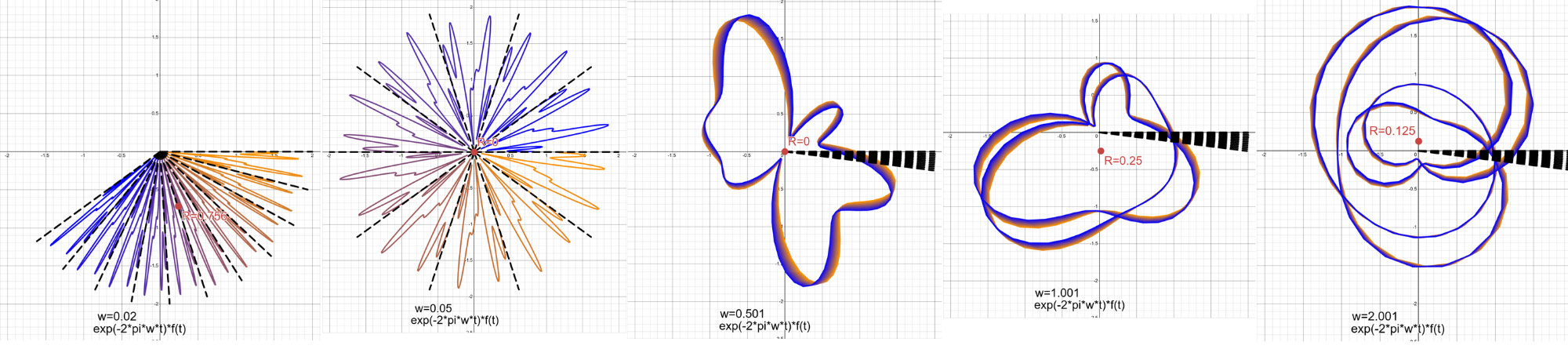
The second step is to find the average value of this polar coordinate encoding of ƒ(t) in terms of the wrapping frequency w. This average value calculation is important because if some frequency w₀ happens to be an important part of ƒ(t), then at w = w₀ the peaks and valleys will line up constructively in such a way that this average value is pulled away from the origin. If however, w₀ is not relevant to ƒ(t), then the peaks and valleys will interfere with each other which will cause the polar encoding average point to be very close to the origin. This average value point is shown by a large red dot in each of the Figures 2 through 6. Figure 7 shows a plot of the distance this average value point is away from the origin as a function of the wrapping frequency from w = 0 to w = 5. From calculus, it is known that this polar encoding average value is defined by

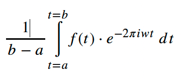
The next step to define the Fourier Transform F(w) is to introduce an interval dependence to this average value point. As it is presently defined, an interval of length 10 seconds and an interval of length 1000 seconds will produce the exact same average value point, assuming the function continues to be periodic. This behavior is not desired because a greater length of measurement in time should produce an equally greater degree of confidence in the frequency information. This change is accomplished by multiplying the average value by the length of the interval b – a.

Finally, taking the limit as the size of the time interval expands indefinitely yields the true definition of the Fourier Transform

Here is a summary of some important facts about this transform:

• The Fourier Transform takes in a real valued function of time, ƒ(t), and returns a complex valued function F(w) in terms of the wrapping frequency w.
• F(w) is symmetric, so F(-w) = F(w).
• The transform is linear, which allows for decomposition into and superposition of simpler functions.
• Plotting |F(w)| shows the relative frequency information contained in ƒ(t).
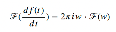
• It turns differential equations into polynomial equations using the fact that $\mathcal{F}\left(\frac{df(t)}{dt}\right) = 2\pi i w \cdot \mathcal{F}(w)$.
• It turns convolution, a difficult problem involving mixing functions, into simple multiplication, which is much easier.
• In most cases, this transform together with its inverse transform converge nicely. It is possible to construct mathematically pathological exception cases, but this is outside the scope of this paper and they almost never show up in real world signals.

Fourier Series

Whereas the Fourier Transform is defined for an unbounded interval, the Fourier Series is only concerned with a particular finite interval [a, b] of length P = b – a. The function ƒ(t) is assumed to be periodic with period P outside this interval. The result of this assumption is that the only nonzero frequency information occurs whenever ƒ(t) is wrapped an integer number of times around the unit circle. If ƒ(t) is wrapped around the circle some fractional number of times, then every k successive cycles of ƒ(t) will combine together to exactly cancel out the average point. This assumption of perfect periodicity also means that the dependence on the length of the interval used in the previous section is no longer needed. We can now define

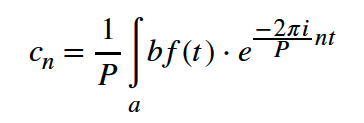
where n is an integer respresenting the number of times that f(t) is wrapped around the unit circle and c_n represents the average value after this n-fold wrapping operation.

With this list of coefficients, c_n, define the following series

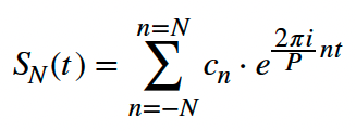
where N is some positive integer representing the maximum value of n. It turns out, rather remarkably, that this series of sinusoids approximates the original function ƒ(t) very well and a higher value of N means a better approximation. S_n(t) best possible approximation of ƒ(t) by sinusoids with frequency less than or equal to $\frac{2\pi N}{P}$ . Look up online the keywords Hilbert Space and Orthonormal Functions for more information about why this approximation works so well.

This series S_n(t) is closely related to the measurement of harmonics in power quality, although the computation details are a little different. All of PMI’s power quality recorders can measure both voltage and current up to the 51st harmonic, or 3060 Hz, in accordance with the IEEE 519 standard.

Discrete Time Fourier Transform

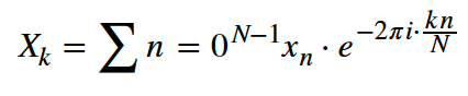
Take the Continuous Fourier Transform, but instead of a continuous input ƒ(t), now consider a sampled input ƒ(nT), where n is some integer and T is the sampling period in seconds. This means that F(w) becomes:

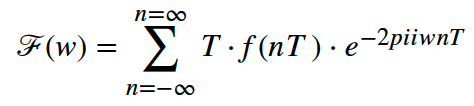
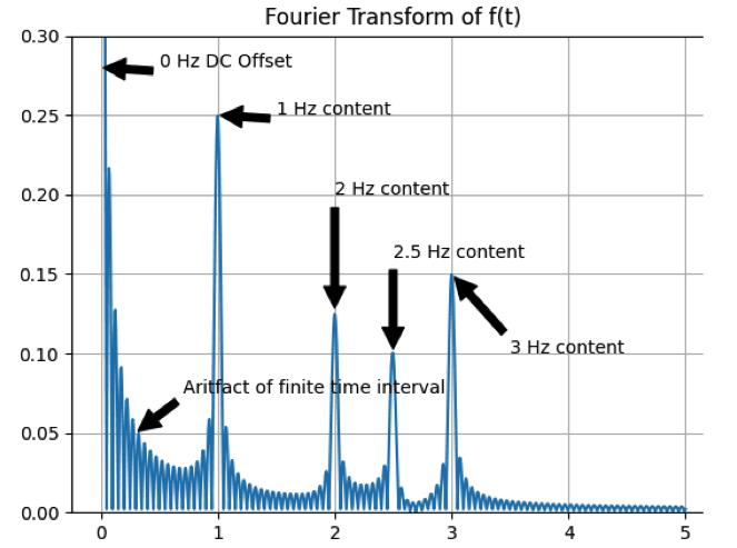
The main difference between this and the continuous Fourier Transform is that the DTFT is periodic in Frequency with period $\frac{1}{T}$. This is because when sampled data is wrapped around the circle, it is possible to wrap it with w₀ radians spaced between each point or 2π + w₀ radians or 4π + w₀ radians or 2kπ + w₀ radians for any general integer k and all of these options look and behave exactly the same. Figure 8 shows the Discrete Time Fourier Transform of ƒ(t), where ƒ(t) is sampled at 25 Hz, which means that the frequency content repeats every 25 Hz.

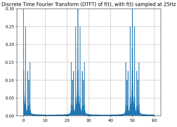
This periodicity in the frequency domain can lead to a problem known as aliasing, where the high frequency content in one band overlaps with the low frequency content in the next frequency band. This overlap leads to distortion when the signal is reconstructed in the time domain and the greater the overlap between the frequency bands, the greater the distortion effect. An important theorem to avoid aliasing is the Shannon-Nyquist Sampling theorem, which says that if a function contains no frequency content higher than B hertz, then the function can be completely reconstructed if it is sampled at or higher than 2B hertz.

This algorithm is used by a PQ recorder behind the scenes whenever it computes the harmonic content of a measured voltage or current signal. The FFT algorithm makes it practical to compute harmonics in real time.

Discrete Fourier Transform

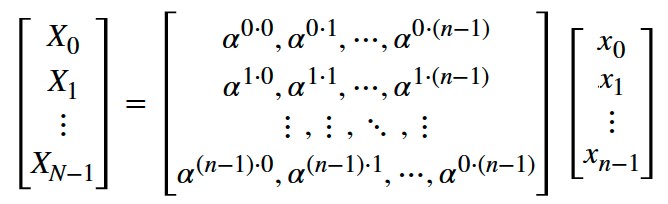
The Discrete Fourier Transform is combination of the previous sections, where we assume both a finite interval and equally spaced sampled points from that interval. We assume that outside the defined interval, the function samples repeat every interval length. This means that resulting frequency domain is both sampled and periodic. Given N sampled points x₀, x₁, …, x_N-1, define the DFT as:

where k represents the integer nuber of times that the points x_n were wrapped around the unit circle. With $\alpha = e^{\frac{-2\pi i}{N}}$, this definition is equivalent to this matrix vector product.

This computation has complexity O(N²), which means that the time required to complete goes up by N² as the number of data points goes up by N. For any reasonably large data set, computing this DFT matrix vector product is essentially impossible to do quickly.

Fast Fourier Transform

The Fast Fourier Transform is a clever implementation of the DFT algorithm which reduces the complexity from O(N²) to O(N · log₂(N)), which dramatically improves performance. If N ≈ 1,000, then the FFT is approximately 100 times faster than the DFT. If N ≈ 1,000,000, then the FFT is about 52 thousand times faster than the DFT. It works by starting with a power of 2 number of points, splitting them into an even index sequence and an odd index sequence, recursively computing the FFT of each smaller sequence, and then recombining those operations. The first $\frac{n}{2}$ points are recombined by $FFT_{even}[j] + e^{\frac{2\pi ij}{N}} \cdot FFT_{odd}[j]$ and the second $\frac{n}{2}$ points are combined by $FFT_{even}[j] + e^{\frac{2\pi ij}{N}} \cdot FFT_{odd}[j]$ .

This algorithm is used by a PQ recorder behind the scenes whenever it computes the harmonic content of a measured voltage or current signal. The FFT algorithm makes it practical to compute harmonics in real time.

Conclusion

Harmonic Analysis is a crucial part of any power quality investigation and observing a signal in the frequency domain allows a power quality engineer to answer many questions about the signal that would be much harder to see in the time domain. The intention of this white paper is to provide some of the necessary mathematical background regarding the Fourier Transform, why it works, and some of its important variations. The core idea behind this transform is to take a function, wrap it around the unit circle, and compute the average value. This transform can be varied slightly by assuming 1) that time domain is periodic implying frequency domain is sampled as in the Fourier Series, 2) that time domain is sampled implying frequency domain is periodic as in the Discrete Time Fourier Transform, or 3) that time domain is both sampled and periodic implying that frequency domain is both sampled and periodic as in the Discrete Fourier Transform. The Fast Fourier Transform is a computationally efficient way to compute the DFT and forms the backbone behind how power quality recorders compute harmonic information.