Abstract

In the previous whitepaper Estimating THD with PF and DPF, a technique for estimating THD was shown given power factor and displacement power factor stripchart data. In many case, there’s no need to record both PF and DPF stripcharts. Without both recorded, it’s impossible to estimate THD with that technique. However, cycle histogram data for PF and DPF are always enabled, and thus available in any recording session from a PMI PQ recorder that can measure power. A method is presented here to use this histogram data to estimate average harmonic distortion for an entire recording session.

Theoretical Background

True power factor is computed from the real power, and the RMS voltage and current values:

where W is the real power over at least one cycle, and VA is the apparent power, or RMS voltage times RMS current. All three components in the PF formula use the entire instantaneous waveform, including all harmonic and interharmonic components.

Displacement power factor (DPF), is the “power factor” of the 60 Hz fundamental, computed as the cosine of the phase angle between the current and voltage fundamental sine waves:

The DPF measurement only takes into account the 60 Hz fundamental. No harmonic and interharmonic components are included, and the DPF reading does not vary with their levels.

This difference in PF and DPF – the former includes harmonics, the latter excludes them – forms the basis for estimating the presence of harmonics without any explicit harmonic data. As described in the earlier whitepaper, an empirical formula was developed to estimate the composite voltage and current THD from the measured PF and DPF values:

This estimate can be useful, but is subject to the following caveats:

• It doesn’t separate voltage THD from current THD – the estimate is actually a composite of the two. Normally the current THD is dominant though.
• It was derived from a waveform with a specific harmonic pattern, and thus may not be as accurate with other distortion patterns.

Nonetheless, the formula provided a reasonably good estimate with several test files in earlier tests with stripchart data.

Using Histogram Data

Unfortunately, stripchart data for both power factor and displacement power factor are not always available. Frequently there is no need to record both types of power factor readings at the same time, especially in cases where harmonics are also not recorded. With older recorders that may not have harmonic options, conserving memory by disabling unneeded stripchart measurements is commonly done, and often will result in a lack of either PF or DPF readings.

All PMI recorders that can measure power keep cycle-resolution histograms of real, reactive, and apparent power, along with power factor and displacement power factor. Unlike stripchart data, histograms are a small, fixed-size data type, and thus there is little penalty in memory consumption for keeping them enabled. For this reason they are always enabled in PMI records, and can be used for some basic analysis even when stripchart data is not present.

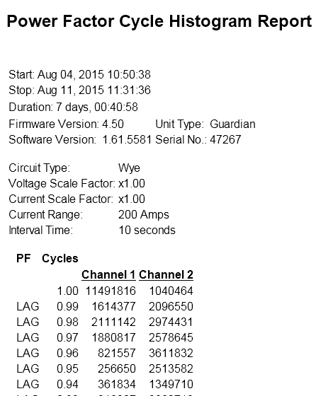
The cycle histogram reports are used in this analysis; to access them go to Reports, Single Cycle Histograms, then choose either Power Factor or Displacement Power Factor. An example for Power Factor is shown in Figure 1 for a 2 channel Guardian recorder. The power factor ranges from 1.00, through 0.99, 0.98, etc. LAG, then further down the report the LEAD values begin at 0.01 and finish at 0.99. The number of power line cycles spent at each PF value is accumulated for each channel during the recording. In Figure 1, the power factor for channel 1 was 0.96 LAG for 821557 cycles in this 7-day recording. 821577/60/3600 = 3.8 hours of total time at 0.96 PF. The nature of a histogram removes all time series information though – there is no way to know when those 821577 cycles at 0.96 LAG occurred over the 7 days – it could have been 3.8 consecutive hours, or 821577 scattered cycles all through the recording session. The lack of any time information means that estimates created from histogram data are necessarily averages over the entire recording session. This is true for average PF and DPF, as well as the estimated THD values.

To use the PF and DPF histogram for a THD estimate, both histograms must be exported to Excel. This may be done by right-clicking the report and choosing to export in Excel or CSV format. Once exported, load the Excel master sheet for this analysis (available for download here), and copy/paste the columns for each histogram into the master sheet. Paste the PF data start at column A1, and the DPF data starting at column H1 (paste directly over the two cells labeled “PF data goes here” and “DPF data goes here”). The result should appear as in Figure 2.

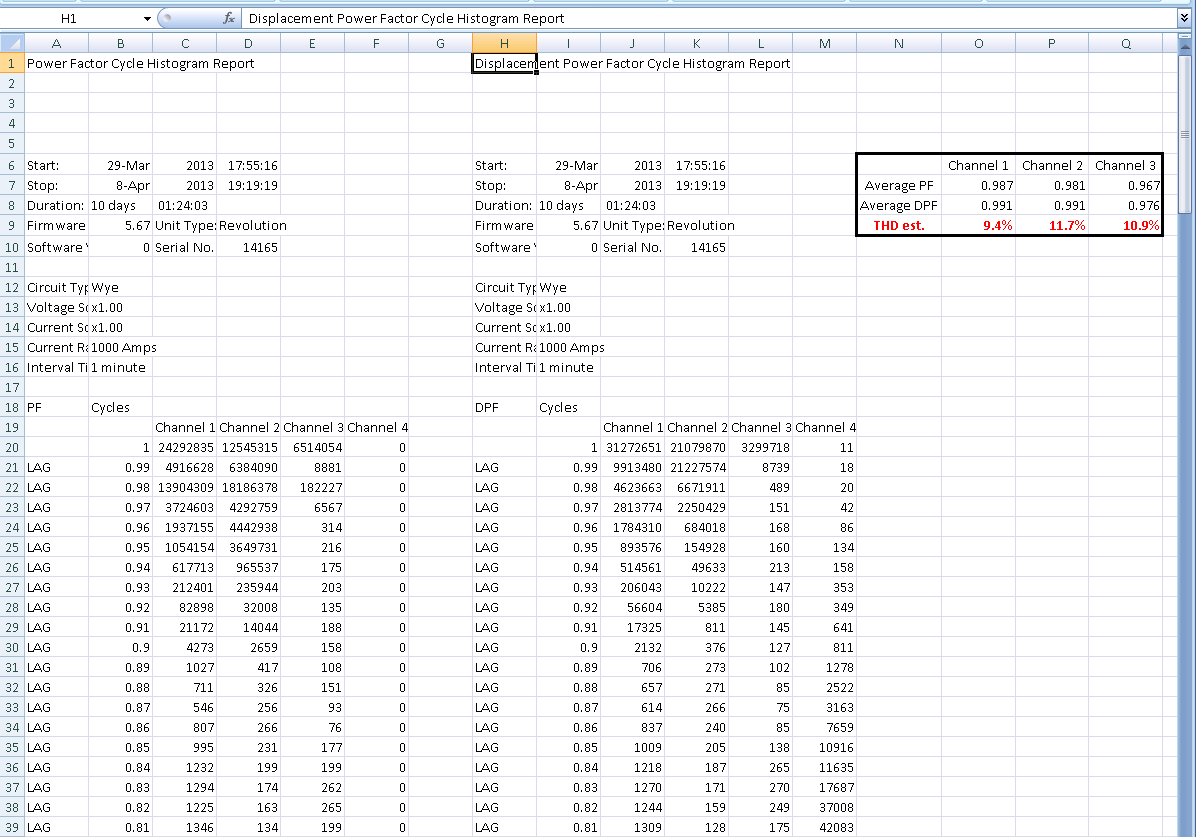
On the right side of the spreadsheet (inside the black bordered area) are average PF, DPF, and THD values for channel 1, 2, and 3. This method is only valid for channels with meaningful power factor and displacement power factor values, so channel 4 THD, usually used for neutral or ground monitoring, cannot be estimated here.

The “Average PF” and “Average DPF” values are computed by summing the product of each histogram bin with the specific bin count. This sum is then divided by the total number of all bin counts (in other words, the total number of cycles in the recording). This is essentially a weighted average of all possible PF and DPF values (1.00, 0.99, 0.98, etc.), with each value weighted by the total number of cycles at that value. As an example, the Excel formula for average PF for channel 1 in the sheet is

SUMPRODUCT($I20 : $I220, J20 : J220)/SUM(J20 : J220)

which computes the weighted average

where i ranges from 0.99 LAG to 0.99 LEAD (and also values 1.00 and 0.00, which are technically neither leading nor lagging, and BIN_i is the i^th histogram bin count.

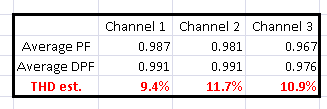
A close-up of this section is shown in Figure 3. Here the average PF and DPF values are computed for channels 1, 2, and 3. The values are close to ideal, and there is a small separation between PF and DPF. The THD values from the formula above are computed the “THD est.” row. In the example here, the values are 9.4%, 11.7%, and 10.9% for channel 1, 2, and 3.

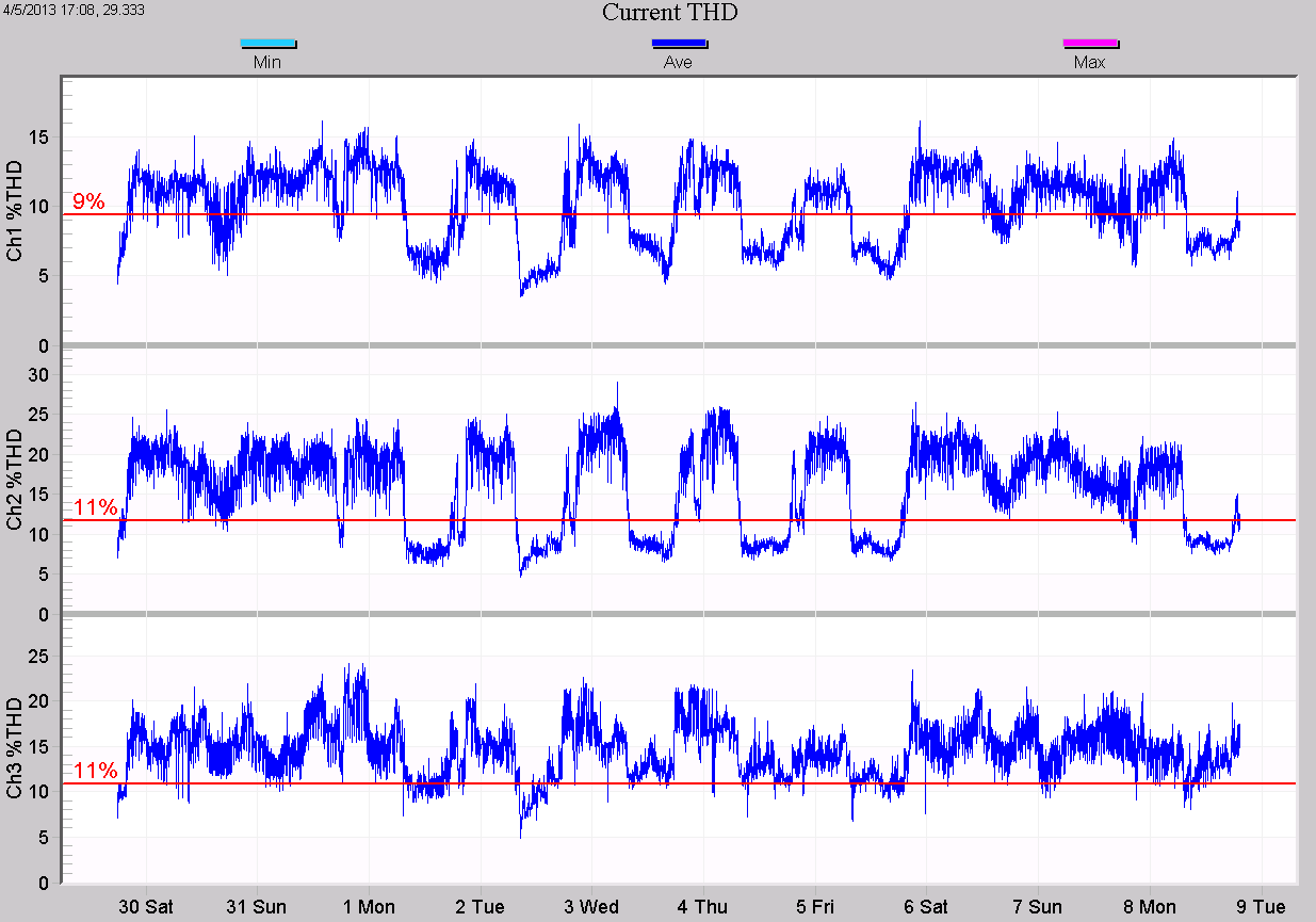
It’s important to note that these estimates are single values for the entire recording session, and also a composite of the actual voltage and current THD (it’s not possible to estimate them separately with this method). Even with these limitations useful information is provided. In this recording, real THD information is available, and in Figure 4 the current average THD values for the entire recording are plotted. The estimates from Figure 3 are annotated with horizontal red bars. The estimates are roughly in line with the average THD, with channel 1 showing as a little lower than the other channels. In this recording, the real THD is lower during the day and higher at night and weekends (resistive load present during the workday improves the THD relative to the background harmonic loads). With a varying THD, the value will swing above and below the average estimated in Figure 3.

Examples

A single-phase example is shown in Figure 5. Only the first two channels have useful data in this recording. From the spreadsheet in Figure 5:

Channel 1: Average PF 0.792, Average DPF 0.979, THD Est. 65.5%
Channel 2: Average PF 0.927, Average DPF 0.928, THD Est. 8.6%

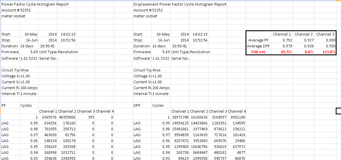
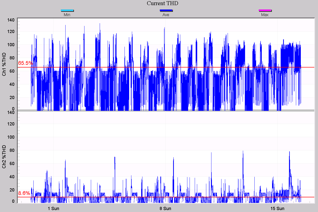
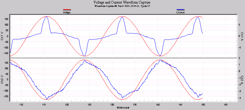
The channel 1 PF and DPF estimates are quite different, while channel 2’s values are very close. Consequently, a high THD is estimated for channel 1 only. Actual THD was recorded in this case, and those measurements are shown in Figure 6 with the estimated THD values annotated in red. Channel 1 really does have a high THD level, and 65% appears to be a good overall average. If THD were not available in this recording, it would still possible to conclude that one leg has a high THD, and that given the single phase service it’s likely due to a load at this customer. Fortunately waveform capture is also available in this recording, and a quick peek at a sample waveform (Figure 7) shows that the channel 1 current waveform is much more distorted than channel 2, corroborating the stripchart data and also the histogram analysis. Note that the specific waveform distortion shown is significantly different than the distorted shape used in the earlier white paper for empirically determining the THD estimation formula, yet the estimated values here are still good. This demonstrates the insensitivity of the method to the specific harmonic distortion pattern.

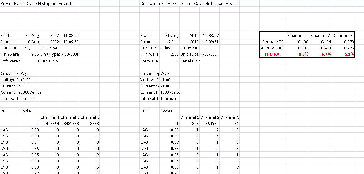
A final example is shown in Figure 8. This file is from an iVS-3/600P, a recorder which can measure power, but has no harmonic or waveform capabilities. The spreadsheet estimates for average THD are 8.8%, 6.7%, and 5.1% for channels 1, 2, and 3. It’s impossible to verify that these are correct, but it’s very likely there was no harmonic issue at this location.

Conclusion

A method was shown to estimate THD in recordings where no harmonics or waveform data is present, even with no stripchart PF or DPF data. This analysis is possible from the fact that true PF contains implicit harmonic information from the real and apparent power values, while DPF is harmonic-free. PF and DPF histograms are always enabled in PMI recorders that can measure power. These histograms can be analyzed to estimate an average THD for the entire recording. Although only a single average THD over the entire recording for each channel can be estimated, this still provides useful information on whether a follow-up recording with harmonics is needed, or to compare with a more recent recording at the same location.