The cycle histogram is an important, but underused record type available with all PMI recorders. The histogram doesn’t require any configuration, spans the entire recording session (no possibility of memory overflow), has cycle-level resolution, and is always enabled. Histograms are traditionally used for statistical analyses, and since all time information has been removed, it is not usually thought of when event duration or analysis is required. This paper shows a way to use the histogram for cycle-level event duration calculation without using waveform capture or other more advanced record types.
A histogram is a graphical classification of data into bins. The RMS Voltage Cycle Histogram includes 600 bins, one for each integral voltage reading – that is, a bin for 0V, 1V, 2V, … all the way to 599V. Every cycle, the RMS value is computed, and the bin count for that voltage reading is incremented. Each cycle one of the bins must be incremented, and over the entire recording session every single cycle is counted in a bin. (See the whitepaper Histograms in ProVision for more on histogram basics). Since each bin is just a numeric count of the reading at that level, all time information seems to be lost. With a little knowledge of the monitored load, it’s possible to get some of that back.
To illustrate the technique, a short test recording was created with a Revolution and a programmable AC power source. The Revolution was fed a steady 120V RMS voltage, except for a 24 cycle sag in the middle of the recording. The sag voltage was 84V, or 70% of nominal. Figure 1 shows the RMS Voltage Interval Graph, with the minimum voltage around 84V during the sag. No indication of how long the sag lasted is given here though. For this test, waveform capture was available, and the event was easily caught (Figure 2). The long sag duration created two waveform captures – one for the start, and one for the end. By subtracting the timestamps (circled in Figure 2), the event is seen to last 24 cycles.
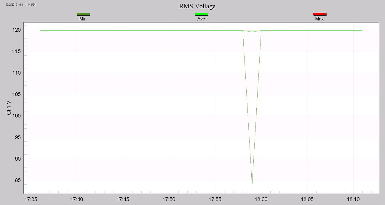
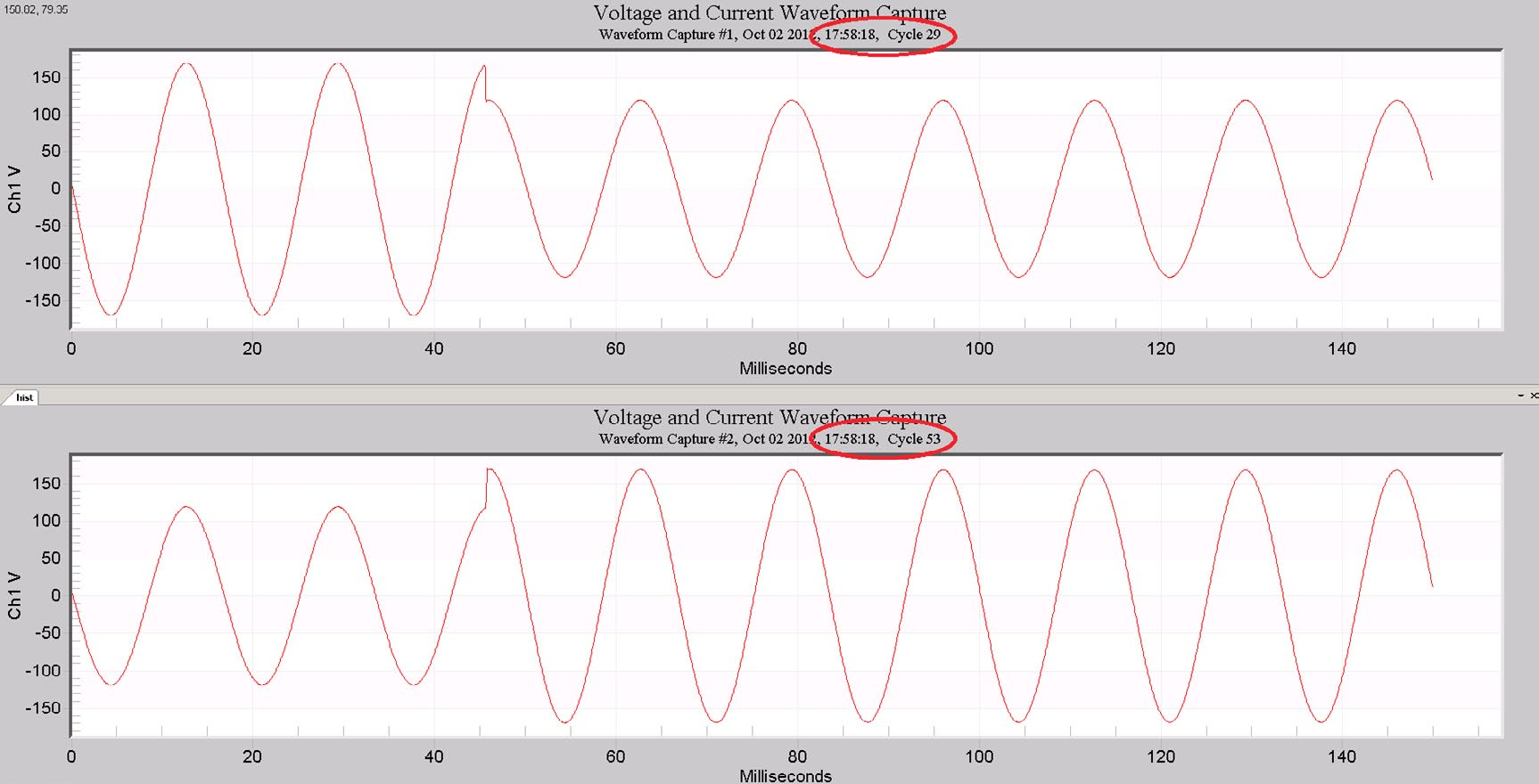
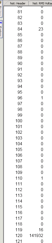
Figure 3 shows a section of the RMS Voltage Cycle Histogram. The first column is for the RMS Voltage bins, and the second column is the bin count for channel 1. Here we see 141,932 cycles for 120V, 16 for 119V, 1 each for 110 and 96V, and 23 cycles at 84V. If we add up all the cycles, the total, 141,972 cycles, should equate to the entire recording time – in this case, 39 minutes, 26 seconds. We know that there was only one sag during the recording (confirmed by the Interval Graph in Figure 1). Thus, all 23 cycles at 84V must have been during that sag, therefore the sag itself is at least 23 cycles long. The isolated cycle readings at 110V and 96V were likely the RMS values during the sag transition time, and together constitute another cycle of sag time, for a total of 24 cycles.
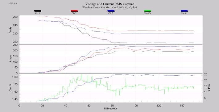
Next, let’s look at a real-world example. An Excel file, containing the associated data, can be downloaded by clicking here. In previous whitepapers, Computing Event Duration with Interval Data, parts I and II, a recording was presented with data from two pumps on a 240V delta circuit. The larger pump’s starting current is over 400A, and pulls the voltage to under 200V (17% sag). The smaller pump draws 200A during the start, pulling the voltage to 220V RMS (8% sag). As shown in the earlier whitepapers, the larger pump’s starting current lasts around 16 cycles. The sag time is easily found by looking at the waveform capture timestamps, but a careful analysis of the interval data gave the same result. However, the smaller pump’s sag time is not apparent in the waveform data. Most of the waveforms are from the larger pump, and those caught from the small pump are from the beginning of the sag, and don’t include the end (Figure 4 shows a typical RMS waveform graph). The small pump’s transition from starting current to running current must be gradual enough to not trigger a waveform capture.
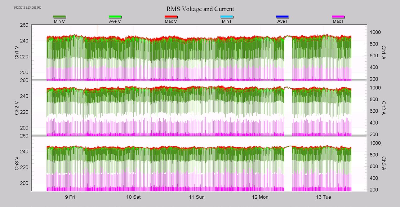
A cursory inspection of the interval data for the entire recording (Figure 5) and a typical section (Figure 6) show that essentially these two pumps are the only load, and most of the voltage variation is due solely to the pump starts. In addition, it’s clear from Figure 6 that the big pump and small pump are distinct in sag voltage – the big pump is always below 200V, and the small pump always above 200V. This is enough information to use the cycle histogram.
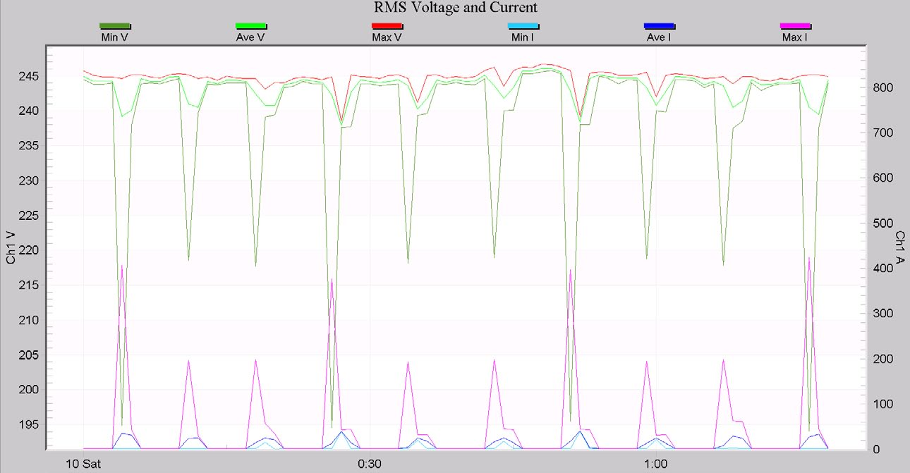
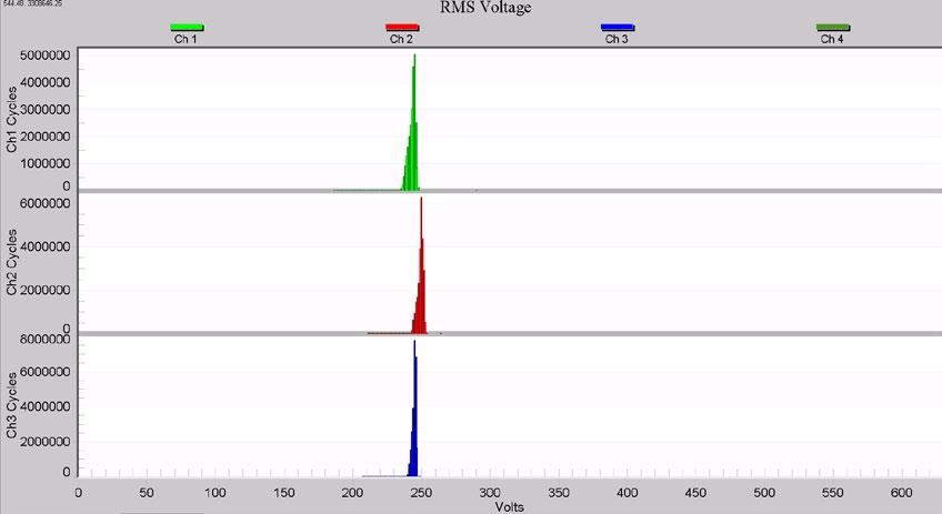
The initial view of the cycle voltage histogram graph (Figure 7) isn’t that helpful, but zooming in on the low voltage section (just visible as a tiny row of dots to the left of the voltage peaks) reveals more. In Figure 8, the two lumps for each phase are centered around the sag levels for the large and small pumps. We also see some unbalance in phases, since the lumps aren’t lined up across all phases (Phase A, green, is the most out of line). The structure here in the graph indicates that there’s more information to be extracted, so we turn to the raw numbers.
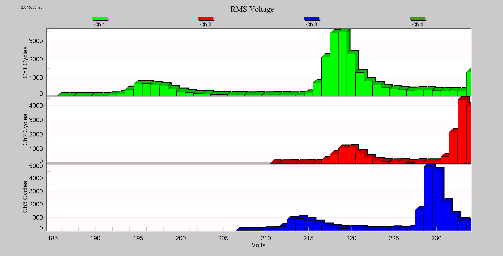
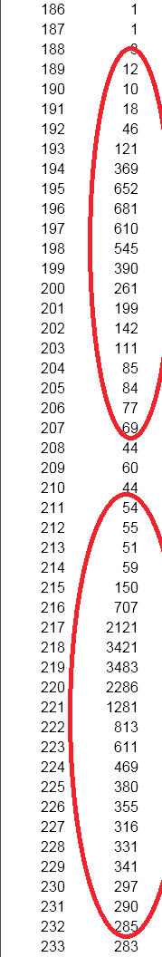
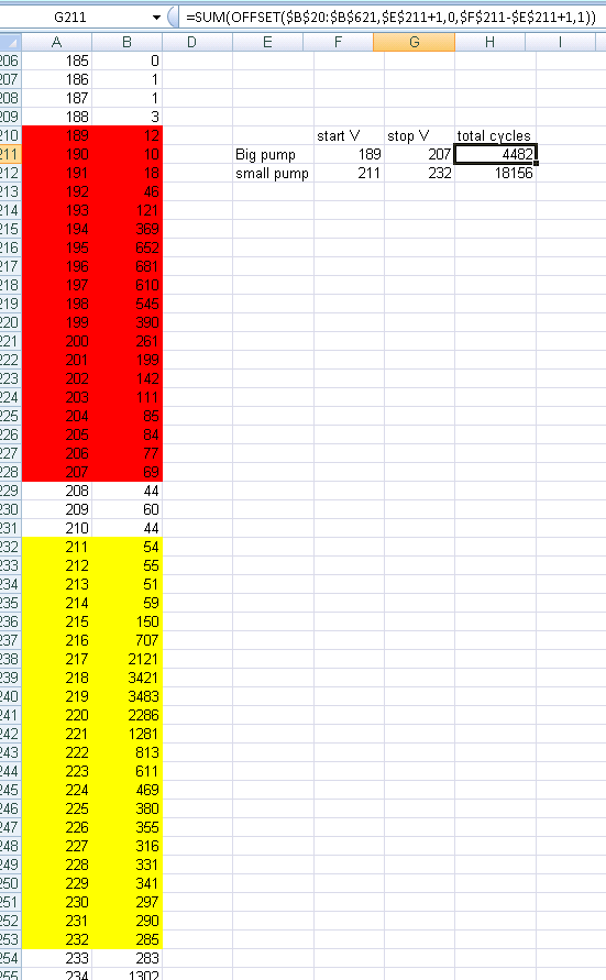
In Figure 9, the RMS Cycle Histogram report is shown for channel 1, with two regions circled in red. The top region, from 189V to 207V, is the sag region for the large pump. The lower region, from 211V–232V, is the small pump, as roughly estimated from eyeballing the numeric lumps. Exporting this to Excel, and entering formulas to automatically compute the total cycles in each region, we can see that the big pump’s total sag time is 4482 cycles, and the small pump’s total time is 18,156 cycles (Figure 10). If we knew the total number of sags, we could divide by that to get the average sag time (assuming the voltage region estimates are correct). In many cases, this information may be known or estimated from outside knowledge of the load, or estimated simply from the interval data. In this file, the situation is complicated by the fact that there are two pumps operating.
Since the stripchart covered the entire recording session, each sag is recorded there by the minimum voltage. Exporting the RMS Voltage Interval Report to Excel, removing all columns except channel 1 minimum voltage, and sorting by that value groups all the sags together. The first 305 entries are sags caused by the big pump, and the sags from row 306 until row 924 look very much like sags from the small pump (see Figures 11 and 12 for close-ups of that section of the spreadsheet). The very sharp boundaries there indicate good estimates of 305 and 619 pump operations for the big and small pumps, respectively.
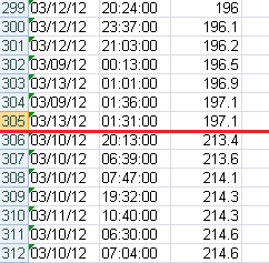
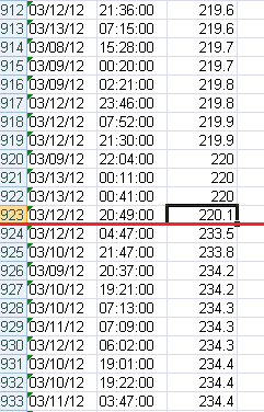
Figure 6 gives a rough cross-check on that – there is one big pump start for every two small pump starts – a 1:2 ratio, agreeing with the 305:619 count.
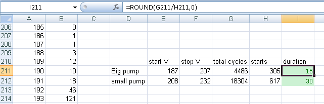
Going back to the cycle histogram data, we can better estimate the voltage ranges for each pump, and divide by the number of events to get average duration. Looking at the cycle histogram, it seems likely that there’s some overlap between the two lumps, that is some cycles between 206V and 213V were caused by both pumps – this could be fine-tuned by using a weighted assignment of counts, based on the relative frequencies of the two pumps, but doesn’t make much difference here. Given the minimum voltages in the interval data from the spreadsheet, the best guess for the big pump is a range from 187V–207V, and for the small pump, from 208V–232V. This gives an estimated sag duration of 4,486/305 = 15 cycles for the big pump, and 18,304/617 = 30 cycles for the small pump (Figure 13).
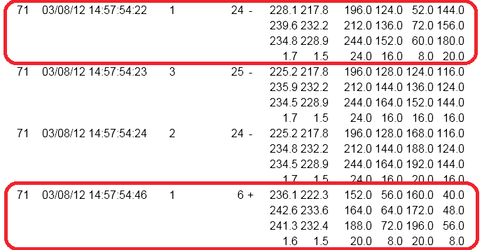
The value of 15 cycles for the large pump agrees closely with the values from waveform capture timestamps and prior analysis in the earlier whitepapers. Unfortunately the small pump’s sag didn’t trigger a waveform capture at the end of the sag, presumably due to a relatively slow return to nominal voltage. The Event Capture Report did catch it though. In Figure 14, the two circled events mark the start and end of a single small pump sag. The sag itself is 24 cycles long, and the return to nominal lasts another 6, for a total of 30 cycles, agreeing well with the histogram estimate of 30 cycles.
Conclusion
Often overlooked, the voltage cycle histogram can be one of the most useful data types for power quality analysis. Present in every PMI recording, regardless of recorder setup or configuration, it logs every cycle in the entire recording session. Normally relegated to statistical analysis, a little extra knowledge of the monitoring situation can enable event-based information to be calculated from raw histogram data.
