Abstract

The Revolution PQ recorder can compute interharmonics in real-time, and also record each one individually as a stripchart. Each harmonic and interharmonic group and subgroup, as defined by IEC 61000-4-7, is also available. Although this is the simplest method for getting interharmonic data, it’s also possible to compute interharmonics manually with raw waveform capture data from other PMI recorders, such as the Eagle or Guardian. This method is also useful for extracting interharmonic data with a Revolution without incurring the memory cost of enabling many individual interharmonics as stripcharts – all 612 interharmonics are available from the waveform data. This whitepaper presents a spreadsheet with the interharmonic calculations, and describes how to use this with exported waveform capture data from ProVision.

Calculating Interharmonics

As described in the paper, Defining Interharmonics, IEC 61000-4-7 defines a method of dividing the spectrum into 5 Hz bands, each band corresponding to a single interharmonic magnitude value. Further, it defines harmonic groups as the RMS addition of the neighboring interharmonics (mid-way down to the next lower and mid-way up to the higher harmonic), harmonic subgroups as the RMS of the adjacent interharmonics, interharmonic groups as all the interharmonics between each harmonic, and interharmonic subgroups as all interharmonics between each harmonic except for those adjacent to harmonics.

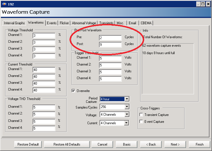
The standard specifies a 12 cycle window for each series of interharmonic calculations. This gives a natural 5 Hz resolution (60Hz / 12 cycles) for the frequency analysis. To mirror this manually, waveform capture should be configured to record at least 12 cycles per capture. The whitepaper Harmonics from Periodic Waveform Capture gives some guidelines for configuring waveform capture for a post-recording harmonic analysis; the only change here is to set the Pre and Post cycles such that the total length is at least 12 (e.g. 2 and 9, as per Figure 1).

Fast Fourier Transform

The heart of the frequency analysis is the FFT, or Fast Fourier Transform. This is an algorithm for efficiently computing the spectrum of a signal. The Revolution performs a 3072 point FFT every 12 cycles (12 cycles at 256 samples per cycle = 3072 samples) as part of the interharmonic process. To compute interharmonics from captured waveform data, the same FFT computation must be done manually. Normally work like this is performed with signal processing package such as MATLAB or Octave, but it’s possible to use an Excel (or Open Office) spreadsheet, which is installed on most office PCs already.

Excel has a built-in FFT macro, but it requires the data length to be a power of two, ruling out 3072 point FFTs. It’s possible to write a VBScript macro in Excel to perform an FFT, but this is very non-portable among different versions of Excel, is often blocked by IT policies, and isn’t available on Macs or with Open Office. The most portable solution is a spreadsheet that computes the 3072 point FFT using only cell formulas – no macros, scripting, or other non-portable methods.

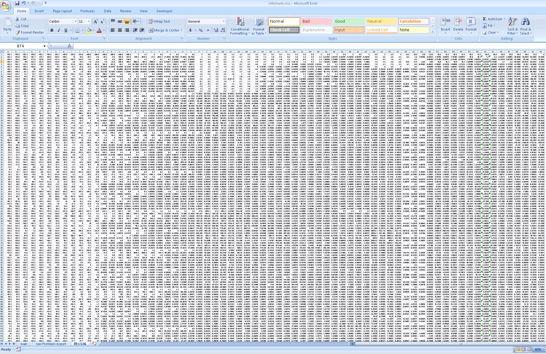
This was created for this whitepaper, and is available for download HERE. It’s composed of three worksheets. Worksheet “fft1536” is the workhorse sheet that contains the FFT computation itself. There’s no need to use this sheet directly; the other sheets refer to it indirectly. This is a 3072-point real-input, complex-output FFT, with the calculations spanning from C1 to BP1536. The input points are in columns A and B, with the points interleaved between the two columns, from rows 1 to 1536. The complex outputs are in columns BO (real values) and BP (imaginary values). In between is a sea of spreadsheet calculations that compute all the intermediate FFT results (Figure 2). Most of the 2.5MB file size is due to this worksheet.

The FFT in the worksheet is actually a 1536-point complex-number transform. In general, a length N/2 complex FFT can be used to compute a length N transform if the input data is real (no imaginary component). This is done by stuffing the even data samples (2nd, 4th, etc) into the imaginary component of the FFT input, and the odds into the real part. In this case, a 3072/2 = 1536 point complex input is created (columns A and B). The raw complex 1536-point FFT output appears in columns BM and BN (real and imaginary, respectively), and are transformed into the 3072-point output in columns BO and BP. Since the input is real, the spectrum is symmetric around 0Hz, and thus there are only 3072/2 = 1536 unique complex frequency components, representing frequency components from 0Hz up to half the sampling rate.

Most common FFT algorithms are designed for an input length that’s a power of 2 (e.g. 2¹⁰ = 1024 points). Unfortunately here the length is 1536 – not a power of two. To handle this length, a mixed-radix algorithm is used, where an FFT of length N can be computed from the combination of two smaller FFTs of length N1 and N2, where N = N1 x N2. N1 and N2 can be further factored recursively until the required FFTs are small and easy to design by hand. In this case, hand-coded FFTs of length 2, 3 and 4 were used as building blocks to create FFTs of length 6 (2×3) and 16 (4×4), then those used for 256 (16×16), and finally 1536 (256×6). These mini-FFT building blocks are buried in columns C to BP, rows 1 through 1536. Each mini-FFT flows from left to right through to the next one, with the original inputs on the left, and final outputs on the right. All this was created by a small program that automatically placed each mini-FFT from the root 2, 3, and 4 sized building blocks, wired them together, and created the master spreadsheet.

Working with Raw Waveform Data

The “raw ProVision export” sheet contains the waveform capture data exactly as exported from ProVision. Copy/Paste the raw data (as described later) here, including all channels of voltage and current. The main worksheet pulls the selected channel from this sheet.

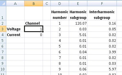
The “main” worksheet is where the desired channel of voltage or current is selected, and where the interharmonic outputs are generated. In the upper left, at B3 and B4, enter the desired voltage or current channel number, and zero for the other (Figure 3). For example, to select voltage channel 3, enter a “3” at B3 (next to “Voltage”), and a “0” at B4 (next to “Current”). Drop-downs lists and other more complex selectors were avoided to maximize the spreadsheet portability.

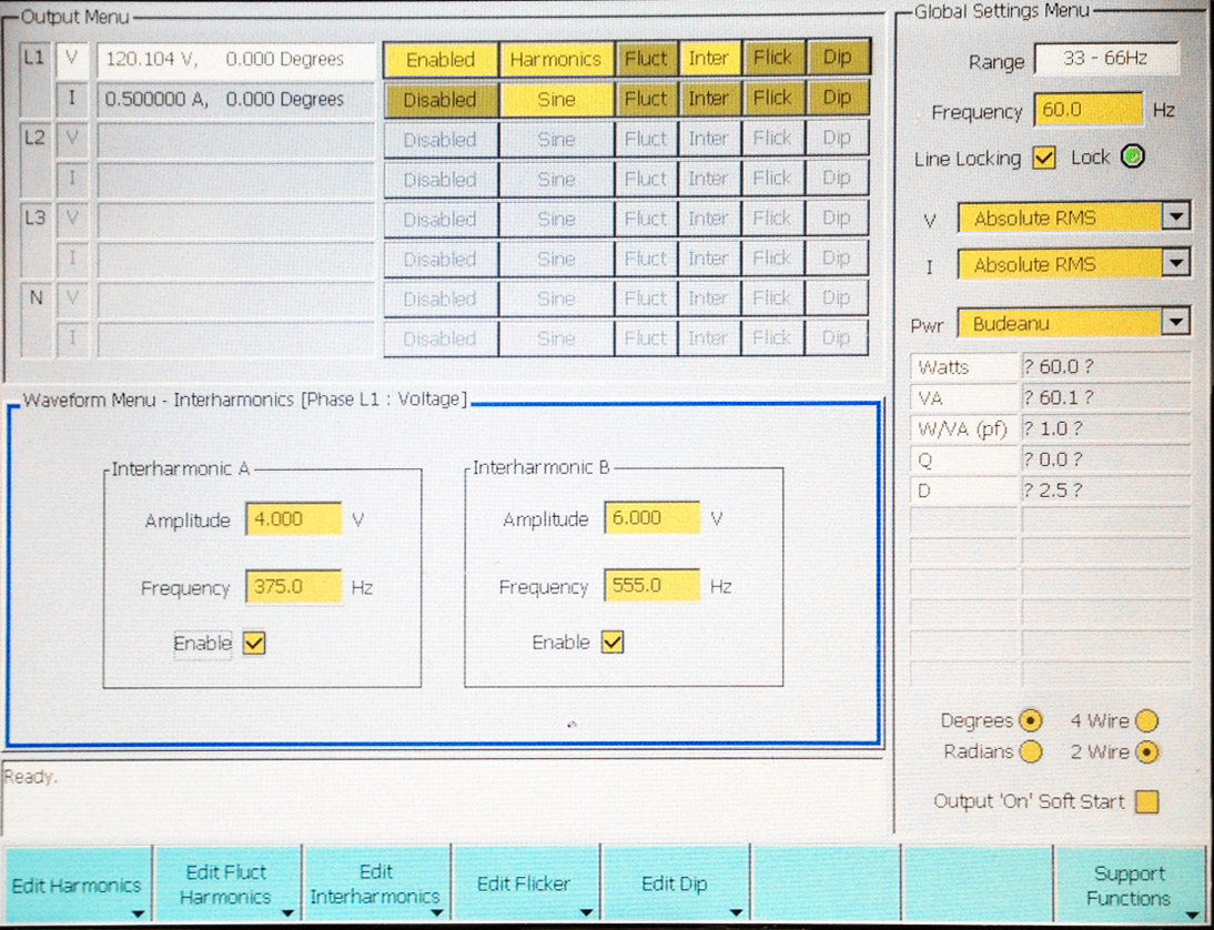
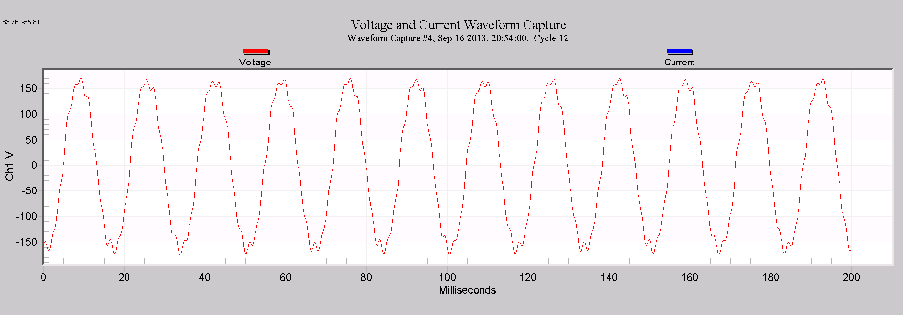
To illustrate the spreadsheet use, a test recording was performed in the PMI lab with a voltage calibration standard capable of generating arbitrary interharmonics. For this test, the values were 5.0V of 3rd harmonic, 4.0V at 375Hz, and 6.0V at 555 Hz (a popular AMR signaling carrier frequency). The resulting RMS value is 120.104V. The interharmonic settings are shown in Figure 4. An Eagle 440 recorded this output on voltage channel 1 with 12 cycle waveform captures every minute. A typical waveform is shown in Figure 5. A waveform capture from this file is contained in the spreadsheet, preloaded in the “raw ProVision export” sheet.

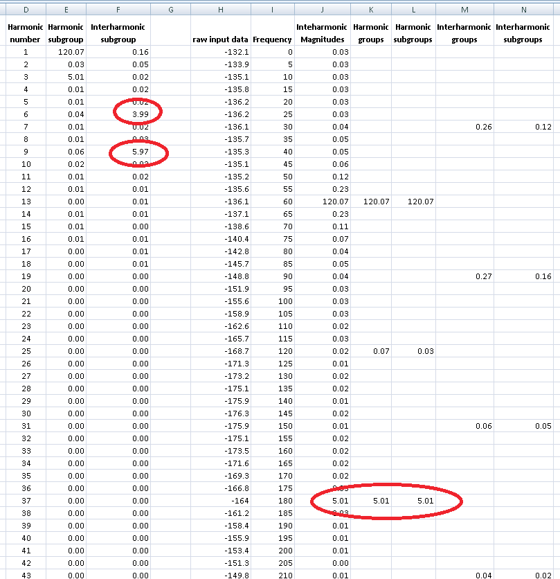
The interharmonic outputs are on the “main” worksheet (Figure 6). The most useful values, the Harmonic and Interharmonic Subgroups, are available in columns E and F. Looking at the 1st, 3rd, 6th, and 9th harmonics, we see the fundamental at 120.07V, the 3rd harmonic at 5.01V, the 6th interharmonic group (including 375Hz) at 3.99V, and the 9th interharmonic group at 5.97V. These agree closely with the voltage generator settings.

The raw interharmonics are available in column J, ranging from 0Hz all the way to 3060Hz (Figure 6). These extend from rows 2 to 613 – they’re spaced 5Hz apart, so there are 612 of them from 0Hz to 3060 (the 51st harmonic).

The harmonic and interharmonic groups and subgroups are in columns K through N (Figure 6). Those are spaced every 12 rows, since there is only one for every 12 interharmonics. The subgroups in columns E and F are consolidated from these columns for better readability. The raw waveform data for the selected voltage or current channel appears in column H; this is the place where the “fft1536” sheet pulls the input data. Normally the selected voltage or current data appears here automatically via spreadsheet references to the “raw ProVision export” sheet.

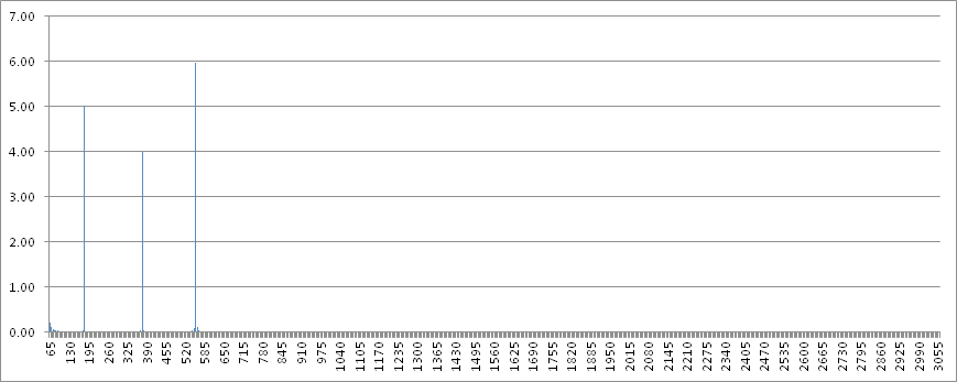
A graph of the raw interharmonics appears to the right of column N (Figure 7), starting at 65Hz. The 5V, 4V, and 6V values at 180, 375, and 555Hz are immediately visible.

The interharmonic calculations and graph update immediately when the channel is changed, or new data is pasted into the “raw ProVision export” sheet.

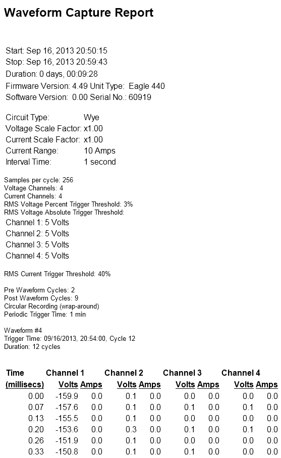
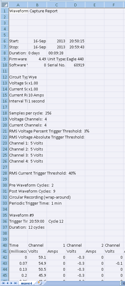
To use the spreadsheet with a new recording, capture some waveforms that are at least 12 cycles long. To export a captured waveform, graph it in ProVision, then choose “Launch Report” by right-clicking on the waveform graph. When the report loads (Figure 8), right-click and choose “Export to CSV”. Save the CSV file to a temporary location.

Next, launch the interharmonic spreadsheet, and also load the saved CSV file with the waveform data. Copy the entire sheet (Control-A, Control-C, or select the entire sheet and select Copy from the menu), then paste it into cell A1 of the “raw ProVision export” sheet – click in A1 of that sheet and press Control-V, or right-click A1 and select Paste (Figure 9). Go to the “main” sheet and enter the number of the desired voltage or current channel, and the interharmonics are immediately generated.

If the raw waveform data comes from another source (a Winscan export, etc.), simply paste the 3072 data points in column H of the “main” sheet – the FFT is computed from whatever data appears there. Pasting values directly in column H will overwrite the logic that uses the voltage/current channel number to pull data from the “raw ProVision export” sheet. The only data requirement is that at least 3072 samples are present, and the sampling rate is 256 samples per 60Hz cycle. A PMI Eagle, Eagle 120, Guardian, Vip, Revolution, or Vision are all possible data sources.

Conclusion

A spreadsheet is presented that computes all interharmonic data from suitable raw waveform capture data. This allows interharmonic analysis from non-Revolution PMI recorders, and also gives some interharmonic ability without using any extra stripchart memory to record all 612 interharmonics. For maximum portability, the FFT is performed only with spreadsheet cell formulas – no macros or plugins are required.