Abstract
The basic formulas for RMS voltage, current, power, etc. in a simple single-phase circuit are well-defined and universal. For polyphase systems, the situation is more complex: in the 3-phase delta there are hidden variables that prevent an exact calculation of some values. For these there are different methods which make different assumptions about the system. Here two different methods for computing apparent power and power factor are given – the arithmetic and vector methods, along with suggestions on which to use.
In a simple single-phase situation, the RMS voltage and current Vrms and Irms, real power W, reactive power VAR, apparent power VA, and power factor PF are straightforward to calculate (see the whitepaper Formulas for Power and Harmonic Measurements for the details). Real power represents the actual power consumed by a load, reactive power is power transferred to and from the utility in a single cycle (but does no net work), and apparent power is the burden seen by the distribution system to deliver the real power (the power “apparent” to the wire, transformers, etc.) Power factor, the ratio of real to apparent power, can be interpreted as an efficiency value, with 1.00 being perfect.
Calculating Apparent Power
These formulas can be extended in the case of a 3-phase wye, since each phase may be treated separately, and a 3-phase total computed from the individual phases. In a 3-phase delta, there is not enough information that can be measured to do this. With a delta, there is no neutral connection, and it’s impossible to measure current “inside the delta”. Since the measured currents are the vector sums of the line currents inside the delta, and there are only two unique voltage readings (the third by definition can be computed from the other two) there is information lost that can’t be recovered mathematically. From Blondel’s theorem, the “two-wattmeter” method may be used to correctly calculate total real power, but it’s not possible to uniquely determine the individual phase power readings. The two-wattmeter method can be extended for total reactive power. Unfortunately, it’s not possible to do this for apparent power—here the concept of total 3-phase apparent power doesn’t have a strong physical meaning, and there are at least two potentially reasonable methods to approximate the “true” apparent power – the arithmetic and vector methods.
Arithmetic Method
The arithmetic method is simply the sum of the individual line apparent powers. This would be mathematically exact, except it’s not possible to unambiguously compute the individual phase apparent powers in the 3-phase delta. One simple approximation is to take the measured RMS voltage and current for each phase and multiply them to get 3-phase VA values. In a perfectly balanced system (equal loads, source voltages, and 120 degree phase angles), these would be too large by a factor of √3, which could then be factored out. In a non-ideal case, the actual factor may not be precisely √3, or even the same for all phases.
A better approach to get individual apparent values is to use the measured phase voltages to compute an artificial neutral point inside the delta. This neutral point is then used to compute synthetic line voltages that are suitable for multiplying directly by the measured currents to get apparent power quantities. In theory, there is always a “correct” neutral point that would produce the correct apparent power readings mathematically, so a good guess for the neutral is the key for this method.
A natural selection for the neutral point is the “center” of the delta voltage vector triangle. If the line voltages are equal and 120 degrees apart, the center of the formed triangle is logical to use as the neutral. In the case of unbalanced systems, the centroid of the triangle is the best. The centroid of a triangle is best visualized as the center of gravity if the triangle were a real object – the balancing point if you were to balance it horizontally at a single point (Figure 1). With a balanced system, the centroid is the center of the triangle, so this seems like a good choice.
The math for computing the centroid, and then the synthetic voltages simplifies quite a bit, resulting in straightforward equations:
where V1, V2, and V3 are the three measured RMS phase voltages. The line-neutral voltages are then used to compute individual phase apparent power:
The centroid method has the advantages of being easy to compute, well behaved (the neutral value is always at least inside the delta triangle and is a “minimum energy” solution from a network theory point of view), and has some physical and geometric meaning. However, the neutral point is still a guess, and not necessarily correct. As will be shown later, the apparent power and power factor computed from this neutral point result in some non-intuitive results from some simple deviations from an ideal system.
Vector Method
The second method for 3-phase delta apparent power calculation is the vector method. Here, the fundamental relation
is used. Since the 3-phase total real and reactive powers can be computed exactly (even in the presence of harmonics), a natural approach is to sum those values and compute total VA from them from
Although this seems like a much simpler approach than the arithmetic method, the actual data processing load to compute real and reactive power is much higher for the vector method, especially if done on a real-time basis.
Under perfect conditions (balanced, equal loads, line voltages, and phase angles), both methods give the same values. As the line voltages or loads become unbalanced, or harmonics are added, they start to diverge. In severe cases the readings can be very different, and the arithmetic method can give very unintuitive results.
Because power factor is computed as real power divided by apparent power, the total 3-phase power factor reading is also directly affected. Often the power factor is of more interest than the apparent power reading, so it’s important to note that the choice of apparent power calculation directly affects it.
The vector method has the pleasing result that the relation
is always preserved, and that for a resistive load, the computed power factor is always 1.00 regardless of the amount of voltage or load unbalance. The arithmetic power factor may be less than 1.00 with unbalanced resistive loads– a non-intuitive result, since power factor is used as a measure of reactive efficiency (which by definition is perfect with purely resistive loads). It’s theoretically possible (although unlikely) for the arithmetic power factor to exceed 1.00, another non-physical result. In general, the vector method more often gives a result closer to what’s physically happening inside the delta, and is numerically better behaved with large unbalances or harmonic distortion.
In the past, the arithmetic method was common due to the lower computational burden (in fact, it’s possible to use analog circuitry without any processing at all), and if anything, was seen as an improvement over simply using the √3 factor arithmetic method. With modern digital sampling and signal processing, the vector method is spreading, but all three methods are still frequently encountered. The arithmetic method is especially common in the form of power factor specifications from motor manufacturers. It’s not unusual for a 3 phase motor controller to have power factor specifications based on arithmetic computations, and these can be quite different than the vector values in the presence of unbalanced voltages, or harmonics. In this case it may be useful to use the arithmetic method to ensure that the measured values match the manufacturer specifications.
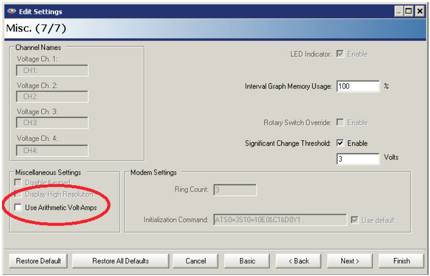
All PMI recorders that can measure power use vector apparent power. With the Revolution and Vision, the arithmetic method is also an option. This choice only affects the apparent power and power factor calculations in a 3-phase delta. Arithmetic power should generally only be used if comparing the results to manufacturer load specifications or other metering devices that also use arithmetic power. Check the “Use Arithmetic Volt-Amps” in the recorder setup wizard (see Figure 2) when initializing a recorder to enable this mode.
To illustrate the difference in readings, a test circuit was created using a 3-phase AC power source, and three resistive loads. The power source was set to create a 120V phase-phase delta (e.g. 69V from line to neutral), and the three loads connected from phase to phase. The three loads were roughly equal values of 21 ohms – nominally 650W heaters. The Revolution was connected as a delta, and the resulting vector diagram is shown in Figure 3.

The balanced power readings are shown in Figure 4, and are the same for both methods. The loads have pulled the voltage from a nominal 120V to 118.8V, and the roughly 118.8/21 = 5.7A current flowing through each resistor is vector added with the adjacent phase to produce √3 x 5.7 = 9.9A measured line current. With this hookup, the total real, reactive, and apparent power, power factor, and displacement power factor are all listed in the Channel 1 column, with the other channels zeroed out.
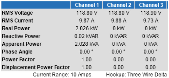
The total power (as seen in the channel 1 column) is about 2kW, and the apparent power is almost identical, with a 1.00 power factor. This is an ideal, resistive, 60Hz balanced delta. Although it’s not possible to determine this from the data, we know that each resistor is roughly equal, so the individual loads are 2.026kW/3 = 675 kW each.
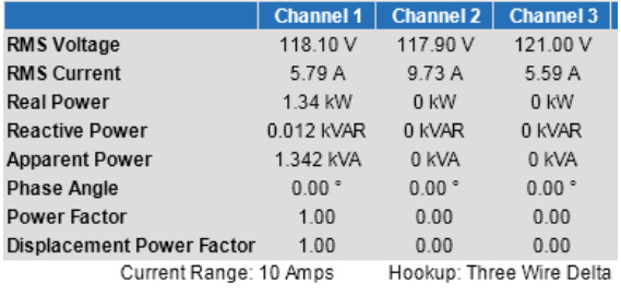
With one heater switched off, the load is no longer balanced. The vector and arithmetic results are shown in Figure 5 and Figure 6, respectively. Both give roughly the same real power (1.34 kW, as expected from 2026 – 675). The vector results still show a power factor of 1.00, which we know to be physically true given the resistive loads. The arithmetic apparent power is higher, and the power factor here is 0.93.

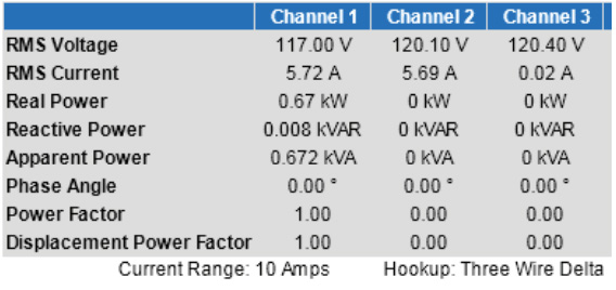
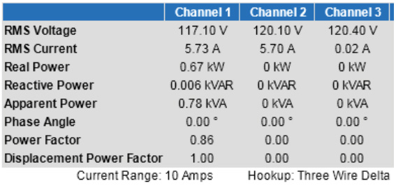
With two heaters off, the load is even more severely unbalanced. The vector and arithmetic results are in Figures 7 and 8, respectively. Again, the real power is correct, but the arithmetic power factor has dropped to 0.86, compared to 1.00 for the vector method. The total load is still 100% resistive, so 1.00 power factor is the better reading – an attempt to “correct” the 0.86 power factor with capacitors would increase the total losses in the system.
Note that the displacement power factor is still 1.00 with both methods. This is computed from just the 60Hz component, and is always made with the vector method. If using arithmetic power, it can be useful to refer to the displacement power factor as a guide to what the vector version would be, keeping in mind that it ignores the presence of harmonics.
Conclusion
An overview of two competing methods for resolving the mathematical impossibility of precisely computing 3-phase delta apparent power was given. The arithmetic method is the older method, but is still seen in legacy meters and from manufacturer equipment specifications. The vector method more often gives intuitive results, and is the default with all PMI power recorders. The Revolution and Vision give the user a choice between the two methods, although the recommendation is for the vector method in most cases, the arithmetic method should be used when comparing readings to like-reading equipment or specs.
