Analyzing Voltage Sags with RMS Capture

Abstract

This white paper covers the topic of voltage sags and a sometimes under-used graphing feature in Provision called the RMS Capture graph. The RMS Capture graph can be very revealing when evaluating and analyzing voltage sags. The RMS Capture allows a user to produce a graph with waveform-level detail without having the scaling problems that occur when using raw sine waves for RMS readings. When there is a measurement need for RMS information, such as analyzing voltage sags, an interval graph does not provide enough detail, and a raw waveform capture plot has an overwhelming amount of detail, along with scaling issues when viewing peak-to-peak sine waves. Here the RMS capture graph may be the best overall view.

Voltage Sags

Voltage sags are one of the most common and costly occurrences that affects power quality. The IEEE defines a voltage sag as a reduction in voltage when to between 10% and 90% of the normal RMS voltage at 60Hz, and when the duration is greater than a half a cycle, or 8.33 msec up to one minute. Voltage sags can be classified by three different types: instantaneous sags, which typically last from 0.5 to 30 cycles; momentary sags, which can last up to three seconds; and temporary sags, which can last up to one full minute. Voltage sags should not be confused with the term brownout, which is a voltage reduction phenomena lasting for a much longer duration than voltage sag, usually lasting for minutes or hours.

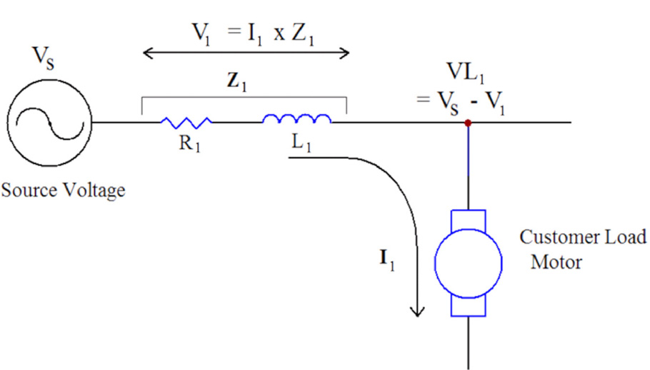
Voltage sags can have many different causes. Anything that can produce a large current by its low impedance compared to the lines’ series impedance in a short period of time can cause the voltage to drop momentarily, causing voltage sag as shown in the schematic in Figure 1. Also, high connection impedances introduced in series with the load, such as a loose connection on a service entrance panel could cause voltage sag issues. Some very common items that can easily cause voltage sags due to their low load impedances are electric motors during their startup sequence, tankless water heaters, arc welders, when a line to ground fault occurs, shorts across the line or lightning causing a line to ground fault. Sometimes voltage sags occur when a transformer connected on the same feed is energized. Refrigerators, air-conditioners, heat pumps, furnace fans, and well pumps all contain electric motors which are major contributors to voltage sags. Some voltage sags are caused by weather-related events such as strong storms with high winds. These cause stress on connections and tree limbs to fall into the power lines along with lightning strikes. Ice buildup on insulators can cause flash-over that can cause sags. Even space weather such as large solar storms can cause voltage sags due to inducing DC on the transmission lines causing transformers to overheat.

Figure 1. Current flow through series line impedance results in voltage drop with large loads

When equipment known to be sensitive to voltage sags frequently malfunctions, it is a good time to install a recorder and take measurements to verify if the malfunction or failure could have be caused by voltage sags or poor power quality. If voltage sags turn out to be the offender, then safeguards can be introduced to protect sensitive electronic against voltage sags.

Mitigation strategies can take one of three approaches. First, the system impedance may be lowered to reduce the voltage drop which causes the sag. Increasing the transformer size or service drop wiring size are good options if most of the drop is occurring there. Frequently most of the voltage drop is inside the building, requiring the customer to address the issue. Second, the high current causing the sag may be mitigated. If a large motor is causing the sag, replacing a hard-start motor with a VFD or soft-start circuit may reduce or even eliminate the in-rush current – thus reducing the voltage drop and the resulting sag. Third, the sensitive load may be isolated from sags with a constant voltage transformer or UPS. This may be the best option if the load is small, particularly sensitive, or if the sags are unavoidable.

RMS Capture

Voltage sags, as with many other power quality issues, are best diagnosed by obtaining the correct information for analysis. RMS Capture is a very valuable tool that can be used to quantify voltage sags on a sub-second and even sub-cycle basis. RMS Capture is useful in determining the change of the RMS voltage or current value over a fixed period of time. RMS capture also has some advantages over interval graphs that do not provide the same level of detail, and sometimes doing raw waveform captures tend to display more detail than is needed to see the larger picture. RMS Capture is only available in ProVision, it is not available in Winscan. Normally, having the most up to date version is of ProVision is preferable, but if you are planning to work with the RMS capture function, version of 1.5 and higher improves graphing speed over the earlier versions. The graphing speed improvement is well worth the time spent to upgrade ProVision the for RMS Capture function.

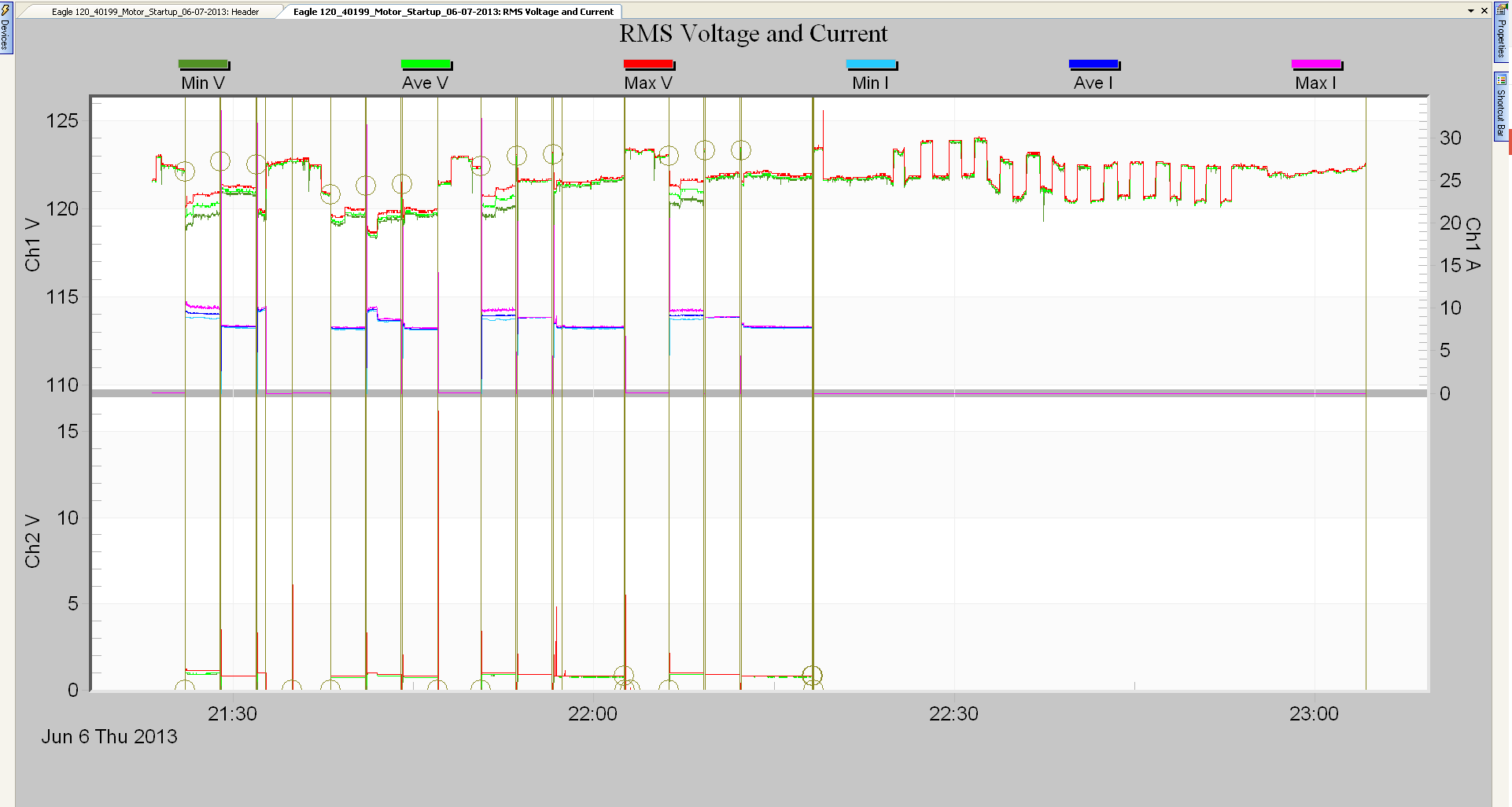
However, most data file analysis begins with the basic RMS Voltage and Current stripchart. This graph provides a good overview of the entire recording session, and is a good launching point for more detailed graphs and reports for specific events. In many cases it’s not known in advance what PQ problem is present, or which captures have the best view of the data, so the RMS Voltage and Current stripchart may be used to begin the file analysis.

To use this feature first bring up ProVision then load the voltage sag file of interest. At this point go to the GRAPH, then RMS Interval, and then to RMS Voltage and Current as shown in Figure 2. It will default to showing the entire recording, with all sags marked via one-cycle min voltage traces. Event captures are marked with circle annotations, and waveform captures with vertical annotations. The stripchart is great for spotting sags and estimating their frequency, but even on the 1 second interval, a voltage sag will be characterized by a single min/max/ave reading. For more detail, the Event Change Table is often the next step. Clicking on a circle annotation in the stripchart will launch the Event Capture for that specific event.

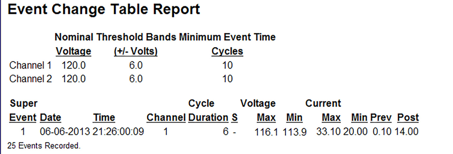
Figure 2 Stripchart graph showing all sags in the recording, with Events marked with circles, and Waveforms marked with vertical lines

In Figure 3, the Event Change Table Report shows the number of events, date, time, channel, cycle duration, maximum and minimum voltage, maximum and minimum current, and previous and post cycles. In the case of this report there was one super event on June 6th, 2015 at 9:26 p.m. on channel 1 for a duration of 6 seconds, with a maximum voltage of 116.1 volts and a minimum voltage of 113.9 volts. The Event Change table shows much more detail than the stripchart, including the sag duration to the cycle level.

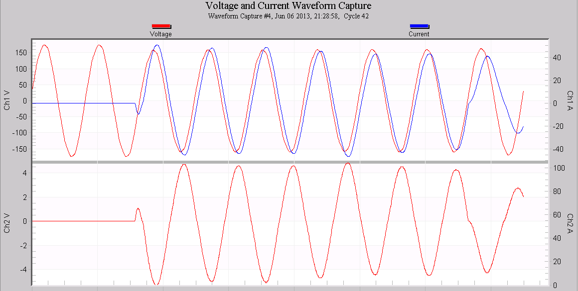
To see even more detail, the waveform capture graph is usually visited next (Figure 4). With this graph, every sample in the event is displayed. Sometimes this level of detail is useful, where the waveshape is important. But with a normal RMS voltage sag, this can be too much detail. Because the plot is scaled to the positive and negative peaks of the sine wave (e.g. -167V to +167V for a 120V nominal), the y-axis spans at least 400V in most situations. A 10% voltage sag is only 12V in a 120V system, and with a 400V y-axis range, a 12V change is very difficult to see. Although waveform capture views are helpful for many other types of disturbances, with an RMS change the details are difficult to see. The waveform graph may be launched from the stripchart by clicking on the vertical annotation, or directly if the time is known for a specific event (e.g. from viewing the Event Capture).

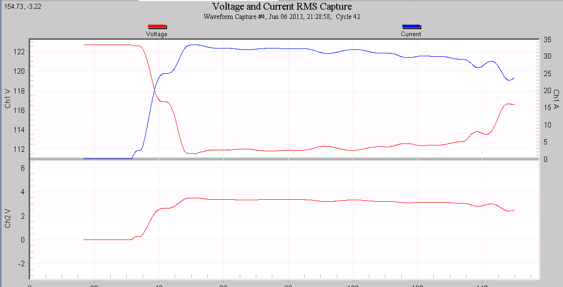
Figure 4. Waveform capture graph. A 10V sag is difficult to see with peak-to-peak sine wave scaling

ProVision can apply a sliding RMS calculation to the raw waveform data to produce the RMS Capture graph, as shown in Figure 5. To generate this graph, choose Graph, Waveform Capture, RMS Capture from the ProVision menu. Choose the same capture event number as the one viewed in the earlier Waveform Capture view. Since only RMS values are plotted, the y-axis spans a much smaller range, and the autoscaling brings out the RMS change instead of hiding it. In Figure 5, the voltage scale has enough resolution to show the RMS voltage sag from a little above 122 volts down to 112 volts. A voltage sag of 10 volts, as the motor pulls over 30 amps, shown in blue, during its start up.

Figure 5. RMS Capture graph of the voltage sag

RMS capture graphs are capable of showing the larger picture of power quality, and by zooming in, can provide high enough resolution to show fine detail. It also clearly shows the relationship between the voltage and current during the voltage sag. Although the RMS Capture graph is not always the best way to view all types of electrical disturbances, it is an ideal way of viewing RMS changes. Because the RMS window is applied sample by sample, sub-cycle resolution is possible, giving even more resolution than the Event Change table.

Whenever possible, it is a good practice to make current measurements along with voltage measurements. The voltage measurement alone can be useful to some degree; however without the current measurement it is hard to evaluate whether the load is the cause of a sag, or just reacting to it from upstream.

Conclusion

RMS capture is a very powerful but underutilized tool that ProVision software provides that is ideal for use in analyzing voltage sags. RMS capture allows the user not to be overly concerned by scaling issues yet allows excellent visualization of RMS changes in both voltage and current. This tool allows the user to be able to view wave-like details in the goldilocks zone, midway between the extremely fine raw waveforms, and the coarse interval graph.