Abstract

Power Monitors provides a range of software tools for power quality analysis, including ProVision, Canvass and PQ Canvass. These general-purpose tools are built towards facilitating the most common types of data analysis among customers. Sometimes more in-depth or customized approach is desired. For these scenarios, PMI provides a full-featured Python 3 library that can be used to extract, analyze and examine power quality data from PMI PQ recordings. This white paper shows how to download and install this library; how to use the library to extract PQ records from recordings; and also highlights some of the built-in utility analysis functions that can facilitate a customized or automated analysis.

Downloading and Installing the Library

Most Python installations ship with a package management utility called pip. This program is typically invoked from the command line in order to install Python packages from a centralized (PyPI) repository. It can, however, be used to install .whl package files that have been downloaded locally. The latter is the primary means of installing PMI’s Python analysis package.

The .whl file can be found at https://powermonitors.com/strip_demo.zip. Begin by downloading this package to an easily navigable directory. Once the file has been downloaded, open a command prompt and navigate to the directory where the .whl file now resides. It can be installed with the following command:

pip3 install --user ./ml_canvass-1.0.5-py3-none-any.whl

This will direct the Python package installer to install the contents of the .whl file for the local user only. In order to make a global installation, the user invoking the pip command must be an administrator.

Note for Windows Users

Since this library depends on a native compiled binary (libnsf.dll) and different Python installations and Windows versions use different default library paths, this library will automatically extract the libnsf.dll (built into the library) into the working directory for each project if the libnsf.dll library does not already exist. This extraction will occur during script runtime for any script that references the nsf_recording class. No special steps need to be taken by the user in order for this to happen.

Library Dependencies

The PMI Python library has two very important dependencies. The pip tool can be used to install them if they are not already present on the system:

• matplotlib – a graphing package for scientific computing.
• numpy – a high-performance library for linear algebra, statistics and other mathematical operations.

Using the Library

The primary module is nsf_recording. This module contains the nsf_recording class, used to read NSF data. The NSF file format is a PMI data format generated directly from ProVision or with a conversion utility (the utility will convert .XSB files to the .NSF format on the fly). See the end of this paper in the Resources section for more information on obtaining the conversion tool.

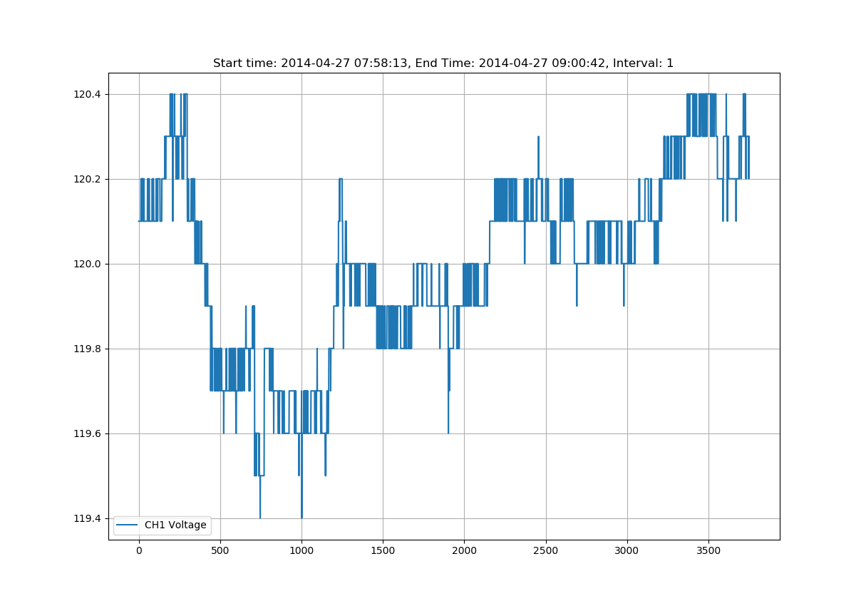
Figure 1 demonstrates how to load and plot a stripchart trace from an NSF file. Figure 2 demonstrates the output of the load_strip.py demo script.

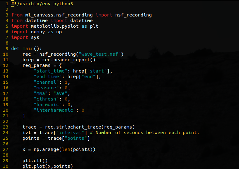
The source for Figure 1 is the resource load_strip.py. The contents of this script will be briefly described below to aid the user in understanding the individual pieces.

The first line of the script, often called the shebang instructs the Linux/UNIX shell to execute the script with the given interpreter (in this instance Python3).

Following (lines 3 through 7) are the imports needed for the script. The first import is used to bring in the nsf_recording class from the ml_canvass.nsf_recording package. This is the primary class that will be used for retrieving PQ data from PMI data files. The remainder of the imports are for graphing, auto-increment array generation, date and time formatting and some system calls.

The main() function is used as the application’s entry point (see lines 41-45 – this forces the Python interpreter to directly invoke the main() function when the script is executed). This function is where all of the useful code is executed.

Line 10 is the instantiation of an nsf_recording object. Note that the only parameter to the constructor is a string, which happens to be the path to the NSF file. This is the only parameter that needs to be passed by users. (There are other optional parameters, such as file mode, but that should not be altered in the event that the write flag is accidentally set.)

The next line (line 11) retrieves the header report object from the recording with a call to the aptly named header_report() method. The return value is actually a hashmap of key-value pairs. It is used to retrieve the start and end times of the recording (which will be passed into the stripchart request).

Lines 12 through 21 define the stripchart trace request. The “start_time” and “end_time” elements are integers in time_t (UNIX time) format. It should be noted that if both are set to 0 and 0, the entire stripchart trace is retrieved. Subsequent calls with adjusted start and end times can be made to retrieve only small portions of the trace if required (ex. if the trace is many millions of points and takes a long time to render).

The channel element is an integer value that is 1-based (i.e. channel 1 = 1, channel 2 = 2, etc.) with a valid range of [1,4]. The measure element is a bit more tricky. It is also an integer value, but is 0-based (it’s actually a C enumerated type). The primary measures that will likely be of use to the user are:

• 0 = RMS Voltage
• 1 = RMS Current
• 2 = Real Power
• 3 = Reactive Power
• 4 = Apparent Power

The “mma” element is an abbreviation of “min, max, average” and allows the user to specify which specific trace they desire. The valid values are “min”, “ave” or “max”.

The “cthresh” element should always remain 0. The remaining elements (“harmonic” and “interharmonic” are self-explanatory. Setting them to 0 disables them.)

Line 23 is the call to the stripchart_trace method of the nsf_recording object. This is the call that actually retrieves the stripchart data. Note that the returned object is a dictionary that contains the following keys:

• interval – number of seconds between each point (this is the stripchart recording interval that was set with ProVision when the recording was initialized).
• decimationFactor – floating point value that is not of use in this application.
• points – an array of point values representing the values recorded in the stripchart trace.

The graphing setup begins on line 27. The call to np.arange generates a series of integer values, starting at 1 and ending at len(points) – 1. These will be used for the x-axis of the plot. Lines 29 through 37 are self-explanatory (clear the plot, plot the x and y values (points), create a grid on the plot, a legend and a title and then show the graph).

Library Documentation

The PMI Python library (ml_canvass) has extensive built-in documentation. This is convenient in that the interactive Python interpreter can be invoked and the built-in help() function can be used to read manpage style documentation for the library.

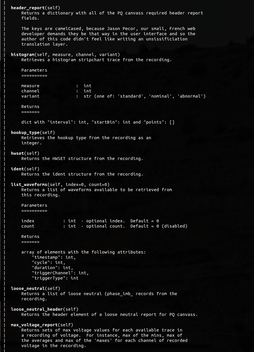
Figure 3 shows how to import the nsf_recording class and browse the help section. Figure 4 shows the actual manpage style documentation that is generated from the library.

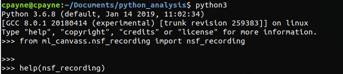
As with man pages, the help screen can be navigated with the standard vi keystrokes (i.e. ctrl+d to page down, ctrl+u to page up, j to scroll down a line, k to scroll up a line and the / character can be used to search for specific methods or text).

Useful Functions

The following is a not-at-all-comprehensive list of some of the functions that are available to the user as part of the nsf_recording class. For more details on parameters and return types, the reader is urged to invoke help(<function name>) from within the interactive Python interpreter.

recording_header() – returns the 4 lines of text that appear at the top of a recording header report in ProVision.

hookup_type() – returns the hookup type that was specified when the recording was initialized.

abnormal_voltage() – returns an array of abnormal voltage events from the recording.

alerts() – returns an array of alerts from the recording.

cbema() – returns an array of CBEMA records from the recording.

events() – returns an array of event capture records from the recording.

flicker() – returns an array of flicker events from the recording.

outages() – returns an array of outage records from the recording.

significant_change() – returns an array of significant change events from the recording.

transient_capture() – returns an array of transient capture records from the recording.

list_waveforms() – returns an array of waveform capture metadata from the recording. This list can be used to select waveforms whose points are to be loaded by the waveform() function.

waveform(index,channel,measure) – returns waveform points and some capture-specific meta-data about an individual waveform capture.

stripchart_trace(params) – returns a stripchart trace. See the examples from figures 1 and 2 above for more details.

energy_usage() – returns an array of energy usage records from the recording.

histogram(measure,channel,variant) – returns histogram record for the specified measure, channel and variant. Variant should be one of ‘standard’, ‘nominal’ or ‘abnormal’ with ‘standard’ being recommended.)

daily_profile(measure,channel) – returns a daily profile trace for the given channel and measure.

loose_neutral() – returns a list of phase imbalance records from the recording.

max_voltage_report() – returns an array of max voltage records.

out_of_limits(measure,min_value,max_value,mode) – generates an out_of_limits report that is an array of timestamp records where values were outside of the specified min and max values.

total_demand_distortion(ratio,start,end) – calculates the total demand distortion given the specified ratio and start and end times in UNIX timestamp. The start and end values default to 0, which will return the TDD for the entire recording.

header_report() – returns a hashmap of key-value pairs that contain the same information that would be found in the ProVision header report.

close() – closes the recording when analysis is complete.

Detailed Example

A more detailed example of how to use Python and the ML Canvass library to “go beyond” the functionality of ProVision is summarized here. The source code for this example (as well as the demo NSF recording used) can be obtained at the following URL: https://powermonitors.com/strip_demo.zip

Figure 5 shows a short screenshot or code snippet for the included stripchart demonstration code. It is recommended that the reader download the code sample from the URL listed above in order to follow along.

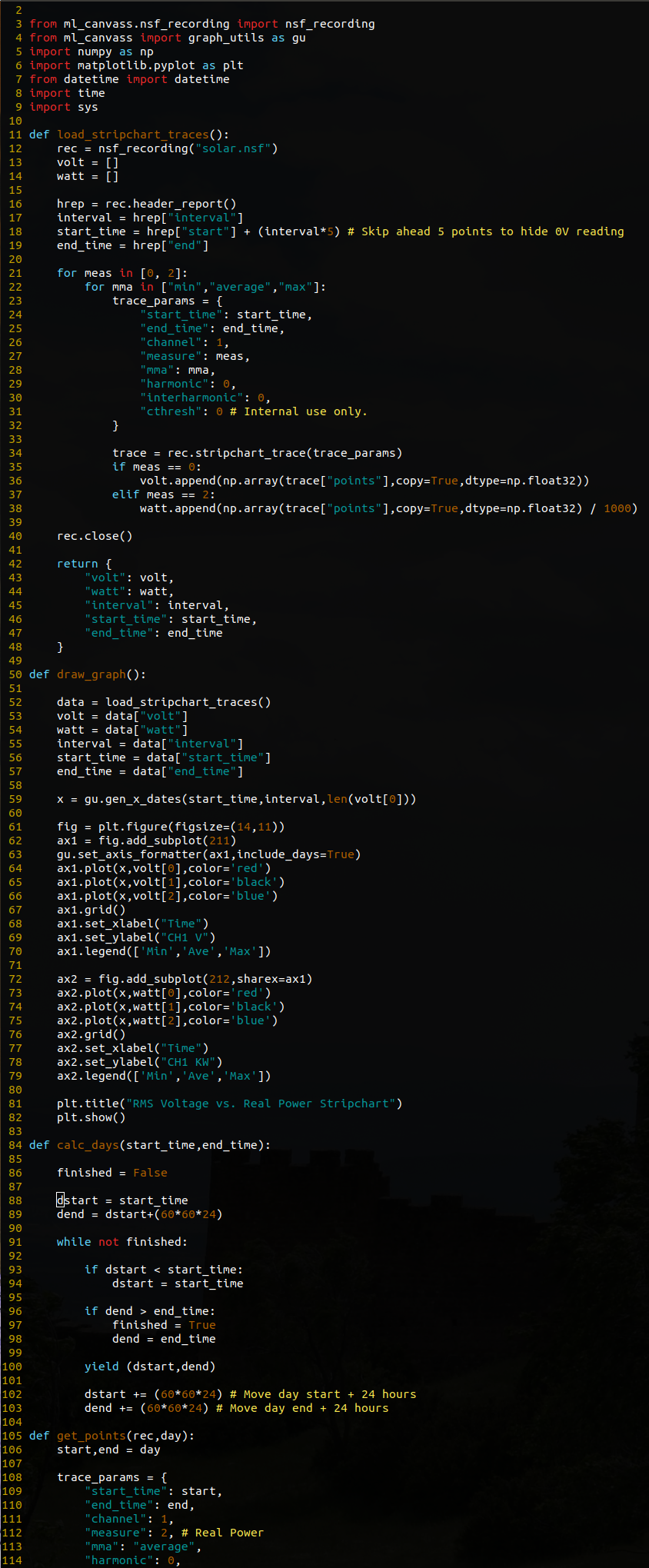
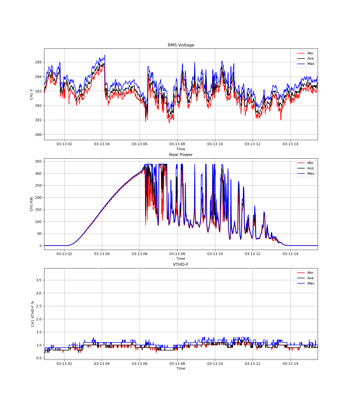
In general terms, this script retrieves the min, average and max stripchart traces for channel 1 voltage and channel 1 real power for the duration of the recording. It then plots both sets of traces (voltage and real power) in two separate interactive plots. (The user is encouraged to zoom, pan, inspect, etc. the graph that is rendered by the application. The interactions are intuitive and the x-axes are synchronized so zooming in on one feature on one plot will force zooming or panning on the corresponding plot.)

The recording is from a solar installation. This data shows the impact of solar generation on voltage regulation during a multi-day span. It is a quick and handy way to show those correlations (and there are several instances of voltage regulators adjusting voltage based on solar output).

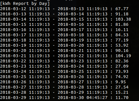
After the first graph closes, the user is presented with a second graph. This graph is a line graph with the calculated kWh per day for each of the 24 hour periods in the recording (except for the final period, which is a fractional day). Closing this graph will result in a console-based text report showing the kWh for each given 24 hour period (from start of recording to end of recording) in a tabular format.

The load_stripchart_traces() function is used to load each of the six stripchart traces (channel 1 voltage min, max and ave and channel 1 real power min, max and ave) from the included recording. The reader will note that there are two loops (one nested within the other) for retrieving these traces – the outer loop to select the measure (0 = voltage, 1 = current, 2 = real power, 3 = reactive power, 4 = apparent power, etc.) and the inner loop to select the “mma” (min/max/average) type for the trace. The resulting points arrays are wrapped in numpy arrays (for ease of mathematical operations), appended to a Python array of return values and then returned as a dictionary with all of the other pertinent recording bits as well.

The next function of interest is the kwh_graph() function. It is used not only to graph the kWh report, but to calculate the kWh values for each 24 hour period as well. This is done through three different functions. The first is a generator function called calc_days() that takes the recording start and end times and generates tuples of 24-hour start/end time periods. Those are passed into the kwh_graph() function when called in the for day in calc_days(start_time,end_time): loop. The resulting real power readings for each individual 24 hour time period is retrieved with subsequent calls to get_points().

Once the points have been retrieved, the total kilowatts for the given period are calculated with a call to np.sum(points) / 1000. That takes the sum of all of the values in the points array and then divides the sum by 1000 (from watts to kilowatts). The next line calculates the actual kWh value by taking kwh = kw / (24 * day_len). The day_len is actually a percentage of a 24 hour day based on the start and end time of the last value from calc_days(). Only the final day is a non-24 hour day, but it’s necessary to use the ratio for each calculation for the sake of accuracy.

Finally, all of these values are appended to an array (along with the start time being appended to a separate x-axis array) so that they can be plotted with matplotlib.

The final section of the kwh_graph() function is used to generate the tabular report of kWh to the console. The source and output of this small loop are fairly self-explanatory.

Conclusion

With the PMI Python data library, a user can easily extract the PQ data needed for further customized analysis. This paper has provided a brief overview of the library’s functionality, an example of how to load data from a PQ recording and suggestions for finding one’s way through the library’s documentation.