Abstract
PMI provides a suite of powerful power quality analysis software packages, from ProVision – the primary desktop offering – to Canvass and PQ Canvass, both web-based products, all well-suited for common PQ analysis tasks. Occasionally a more fine-grained and detailed study is required, especially for unique or experimental situations. In these cases, raw PQ data must be exported from ProVision and analyzed experimentally in more general purpose tools. One such tool is Python, a scripted programming language often used for research data analysis. Here a method is shown to extract and analyze waveform data from a PQ recording using Python and some very common, off-the-shelf scientific computing libraries.
Prerequisites
All of the examples in this document target the 2.7 version of Python. Python 3.6 and 3.7 scripts are available as well for those readers who have decided to use those particular branches. A python runtime (2.7, 3.6 or 3.7) must be installed as well as both the NumPy and Matplotlib libraries (available online, from pip and also bundled with many Python distributions, such as Anaconda Python).
The PMI Python scripts will work on Windows, Linux, and FreeBSD, and require a binary shared library (libnsf.so for Linux and FreeBSD or libnsf.dll for Windows) which is included with the script download (links and references can be found at the bottom of this document).
It should be noted that this is an advanced topic. The reader should be familiar with Python programming before making use of the included scripts.
General Setup and Necessary Files
To get started, download the PMI Python script package (links at the end of the document) for the appropriate platform and architecture and Python version. (Note: Python 3.x scripts are not reverse compatible with Python 2.7 and certain Python 2.7 scripts are not forward compatible with Python 3.x. Ensure that the download selected matches the Python runtime version installed on the target machine).
The download should contain the following files:
- libnsf.[dll or so] – this is the binary library that Python uses in order to read from the PMI recording files in NSF format. This file must be located in the directory with the rest of the Python scripts.
- nsf_recording.py – This is the main Python file that contains the definition for the nsf_recording class. This file must sit in the same directory as the libnsf.[dll or so] file.
- nsf_wave_list.py – This file contains example code for listing all of the waveform capture events in a PMI data recording. The index of these events is used to retrieve data in the other examples. All indices in Python are 0-based, meaning the first entry in the list has index 0, the second entry has index 1, etc.
- nsf_full_waveform.py – This file demonstrates how to pull a full waveform capture event (that can contain multiple cycles in a single capture) and graph all of the captured cycles for the event in the time domain.
- nsf_waveform.py – This file contains an example of extracting a single cycle from a unique waveform capture from a PMI data file. This script also gives an example of performing an FFT on the time-domain waveform values and then plots the time-domain and frequency-domain magnitudes on a split plot graph.
The code snippets for the remainder of this paper will be pulled from nsf_waveform.py.
Analyzing the Script
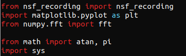
The first import (“from nsf_recording import nsf_recording”) is the most crucial of the imports. This tells the Python runtime to include the source code definitions for the nsf_recording class. The file nsf_recording.py must be in the same directory as the script that is being written.
The remaining import statements (for matplotlib.pyplot and for numpy.fft, etc.) are utility scripts that are used later in our nsf_waveform.py demonstration script.
Main Function
The body of the source code resides in a function called main(). This is to help organize the code layout and to better help it mirror traditional software paradigms where the entry point is a function called main. We will see a little later exactly how this main() function gets invoked by the runtime.
The first executable line of code in this function is declaring and opening a recording object. In this particular instance, the name of the recording is “wave_test.nsf” which is a PMI PQ data file in the NSF format.
Immediately following is a comment block that describes how to retrieve a waveform record from the recording. The method is called waveform and it takes three parameters: The most important considerations are:
- waveform capture index from the recording file. This is a 0-based index, where 0 = the first record
- channel. This is a 1-based value where 1 = Channel 1, 2 = Channel 2, etc. Must be between 1 and 4 inclusive.
- measure. This can be either 0 for Voltage or 1 for Current. No other values will be accepted.
In the line of code that is loading the waveform in our example file, the 2nd waveform capture (index 1) of channel 1 (1) voltage (measure 0) is being retrieved from the recording and stored in a variable called wave.
The wave object is a JSON structure (or Python dictionary) that has the following elements:
- cycle : Integer value that returns the cycle number of the first cycle of data within the capture. Can be between 1 and Max Frequency Hz.
- duration : 32-bit floating point value returning the duration of the waveform capture in milliseconds
- timestamp : 32-bit integer representing the epoch time (UNIX time) of the event. This is the number of seconds elapsed since 1 January 1970 UTC.
- frequencyHz : 32-bit floating point value indicating the measured frequency for the waveform capture
- pointsPerCycle : integer value indicating the “samples per cycle” value. This is the total number of samples (or points) that were stored per each cycle in the waveform capture.
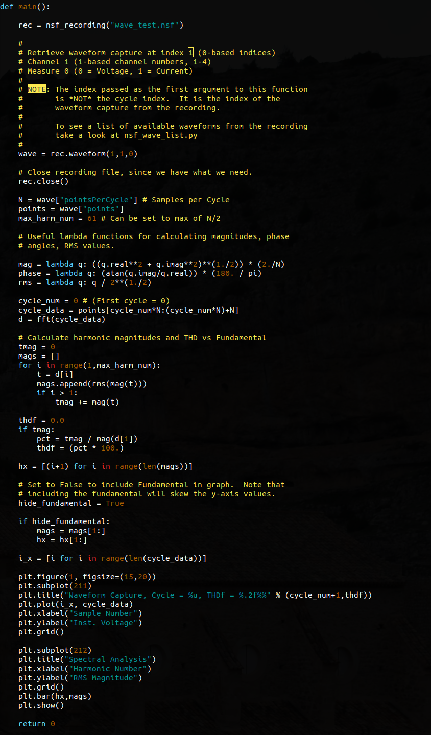
- points : array of floating point values that represent each point in the waveform capture.
After retrieving the waveform record and storing it in the wave variable, the reader will notice that the recording object (rec) is then closed. It is always a good habit to close any file handles that are no longer needed.
Next, a series of variables are declared and set that will be used later in the script.
N = wave[“pointsPerCycle”] assigns the number of points that are measured in each cycle of the waveform capture to a variable called N.
points = wave[“points”] assigns the points array to another variable called points. This isn’t anything special – it’s a convenience. Typing points is easier than typing wave[“points”] repeatedly when the points array needs to be accessed.
max_harm_num = 61 – this line specifies the maximum harmonic number to display. The FFT that is performed later will be N bins in size, where N was declared and defined above as the number of points per cycle. This number (max_harm_num) will be used later when the graph is drawn.
The ** operator is the exponent operator. For example: 2**3 could be evaluated as 2³. The mathematical definitions for each of these lambda functions are as follows:
- The variable q is a complex number with real and imaginary parts. This is because the results of an FFT are complex. This function calculates the magnitude of each bin in the FFT.
- This function calculates the phase angle for each bin in the FFT and converts from radians to degrees.
- Keep in mind that the variable q is a complex number. Python allows scalar operations on all complex numbers, which is why each individual real and imaginary component isn’t divided separately. This function converts the instantaneous magnitudes from the mag expression above into their RMS values.
Selecting a Cycle and Calculating the FFT
The next three lines of code are used for selecting an individual cycle’s worth of data from a waveform capture record, pulling that cycle data out and assigning it to a variable and then computing the FFT for that cycle.
The variable cycle_num is used to define which cycle to extract. Again, since Python is a 0-based index language, cycle 0 will be the first cycle.
The next line is a bit trickier and for some won’t be apparently visible what exactly is happening. The cycle_data variable is being assigned a “slice” (or a subset of an array of data). The values in the brackets in this segment points[cycle_num*N:(cycle_num*N)+N] are specifying the start and end range for the slice. In our example, it is being calculated as follows: 0 * N:(0 * N)+N, which gives us a range of 0 : N. In other words, take the 0th point (the very first point) and give me the next N (remember that N is the number of samples per cycle or “pointsPerCycle” from our waveform record).
Finally, the d = fft(cycle_data) does exactly what it sounds like. An N-point FFT is performed over the variable cycle_data which was just declared and defined one line above.
Total Harmonic Distortion: Calculating the Total Harmonic Distortion (THD) vs the Fundamental
The next block of code is used to calculate the Total Harmonic Distortion of each of the harmonic frequencies calculated from the FFT starting with the 2nd harmonic and ending with the max_harm_num that was declared and defined near the top of the main() function.
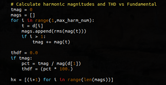
The variable tmag is being used to store the sum of the non-fundamental magnitudes for each of the FFT bins from 2 to max_harm_num. The variable mags is actually an array that will be used to hold the individual RMS values of the magnitudes from the FFT along the range 1 to max_harm_num. This array is used below when the graph is drawn. Note that this array does include the fundamental.
The for loop in this code snippet is used to perform the operations listed above – sum all of the harmonic magnitudes that are greater than the fundamental and append all of the magnitudes (fundamental included) to an array called mags.
thdf is a variable that is used to store the ratio of the sum of the non-fundamental harmonic magnitudes to the magnitude of the fundamental (i.e. THD-F). The code that follows that variable declaration is self-evident.
Graphing the Results
The final section of the main() function is the graphing section. In these few lines of code the data that has been retrieved, calculated and massaged above will be displayed in a matlab style graph. (Python’s Matplotlib library uses a command set that is very close to that of Matlab. If the reader is familiar with Matlab, then the Python code should be very easy to follow.)
The hide_fundamental variable is a convenience added for the reader. Setting this variable to True means that the fundamental magnitude will not be displayed in the resulting graph. This can be useful as the fundamental magnitude is usually many times greater than the remaining harmonic magnitudes and this can cause y-axis scaling results wherein the remaining non-fundamental magnitudes are difficult to visualize.
The code that follows the hide_fundamental declaration is used to “slice out” the 1st element in the magnitudes array.
i_x is an array that is used to generate a sequential series of values corresponding to the length of the time-domain waveform cycle points extracted above (in the cycle_data variable). This will be used for plotting the x-axis of the time-domain data.
All of the remaining lines are fairly self-explanatory. A new graph figure is being created with the given dimensions (figsize=(15,20)) and then subplots are selected. (The 211 value indicates that there are two rows, one column and that the first subplot will be row 1). The second subplot (212) indicates that there are 2 rows, 1 column and that the second row (2) will be selected for the figure.
The only other difference between the two graph commands is plot vs bar. The plot function will generate a line graph, connecting all of the points on the y-axis series together as they progress along the x-axis. It’s a “point-to-point” line graph.
The bar function generates a bar graph at each x-axis location with a y-axis magnitude equivalent to, in our case, the harmonic magnitudes calculated earlier.
Finally, the return 0 value is used to pass an exit code to the interpreter. The Python interpreter will use the system called exit() with this code indicating that the application has terminated normally.
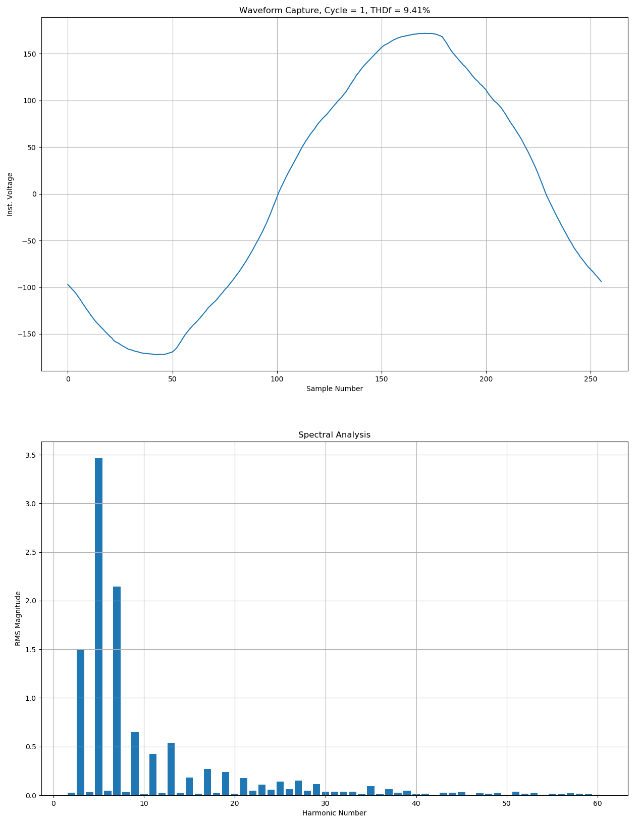
Generated Graph
If the nsf_waveform.py script is run with the included .nsf file (PMI PQ data file), then it will render a single graph window containing two individual graphs: the time series graph for the selected waveform cycle and a bar graph representing the frequency-domain of the FFT results.
Conclusion
The Python programming language is an extremely powerful tool when coupled with the right libraries. This whitepaper has demonstrated how combining Python with a native PMI data library can greatly extend a user’s analysis ability, and provides tools for analyzing raw PQ data with advanced or specialized algorithms.
Reference Links
Each of the following files contains the sources and binaries for python 2.7 and python 3.x.
- https://powermonitors.com/py_pmi_windows32-bit.zip
Description: Windows 32-bit Scripts and Libraries - https://powermonitors.com/py_pmi_freebsd64-bit.tar.bz2
Description: FreeBSD 64-bit Scripts and Libraries - https://powermonitors.com/py_pmi_linux64-bit.tar.bz2
Description: Linux 64-bit Scripts and Libraries
